24µm Focal Plane Survey, Coarse
Principal: Jocelyn Keene
Deputy: Jane Morrison, Bill Wheaton
Data Monkey(s): Jane Morrison, Bill Wheaton
Priority: Critical
Downlink Priority: Normal
Analysis Time: Campaign F: 60 hours, Campaign G: 60 hours, Combined results for F and G: 2 hours
Last Updated:
Objective
To measure the pixel locations (i.e. array orientation, scale and distortion)
as a function of scan mirror angle for the 24µm array.
Description
Use an IER based on the 24 µm photometry AOT for a compact source to measure
the locations on the sky
of several positions on the array as a function of scanning mirror angle.
This task is performed in Campaign F and Campaign G.
After Campaign G is finished the results from campaign F and campaign G are
merged together to update Frame Table # 9.
The frame table updates for all the campaigns can be found in the following
table: Frame Table Updates
Data Collected
IER for 24µm Focal Plane Survey, Coarse collects 336 DCEs, of
which 234 have the source on the array (others will have only much weaker
sources present). The IER is set up so data is collected in 3 columns on the array:
on the left-side, center and right-side of the array. After moving the telescope
in the V direction according to the V offset, the observational pattern is repeated
7 more times (with a V offset between each set).
Calibration Star
See IER for the star chosen. This star was chosen as the 24 µm focal plane
calibrator based on the following requirements:
The star needs to used as the PCRS star as well as the MIPS focal plane star.
Note that PCRS stars have a V magnitude between 7-10 (this catalog is based
on the Tycho and Hipparcos stars).
In the CVZ
MIPS requirements: stellar brightness corresponding to S/N of 30 (3 sec integrations)
at least 14 mJy, K mag 6.53 (range 14 to 500 mJy or K = 6.5 to 1.3)
Observing Strategy
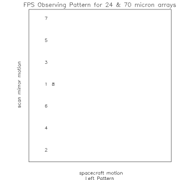
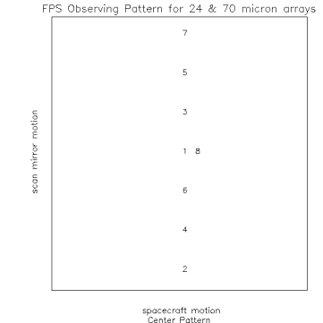
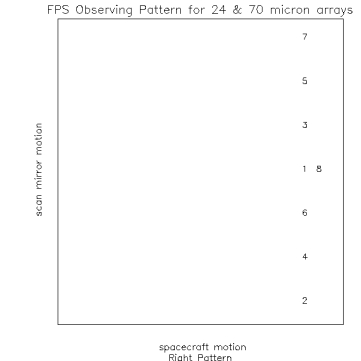
Figure 1. Observing Pattern at 3 locations on the detector. Note size of
box is not the total size of the array but a portion of the central
region which depends on array and if it is a coarse or fine survey
Definitions:
W axis direction is defined by the Frame Table, and is always within +/- 90
degrees of the TPF z axis as projected on the sky. Motion along this axis corresponds to
motion in the spacecraft motion (left/right).
V axis direction is defined by the Frame Table, and is always within +/- 90
degrees of the TPF y axis as projected on the sky. Motion along this axis corresponds to motion
in the scan mirror direction (up/down).
W offset, the amount of motion in the W direction which results in the
spacing between left array, middle array and right array observations
V offset, the amount of motion in the V direction which occurs between a set of
observations.
24 µm Coarse FPS observational parameters:
W offset = 138 arc seconds
V offset = 69 arc seconds
W dither = 3.75 arc seconds
V dither = 3.75 arc seconds
mirror locations for 1 position shown in figure 1.
- position 1 = 0
- position 2 = -69
- position 3 = 23
- position 4 = -46
- position 5 = 46
- position 6 = -23
- position 7 = 69
- position 8 = position 1 = 0
Observational Strategy
Step 1
- PCRS observation
Step 2
- Position the telescope so the data falls on the left side of array
- Take 8 DCES at positions shown in figure 1 (left)
- dither in V and W
- Take 8 DCES at positions shown in figure 1 (left)
Step 3
- Move the space craft according to the W offset (138 arc seconds), image should now
be on the center of the array.
- Take 8 DCES at positions shown in figure 1 (middle)
- dither in V and W
- Take 8 DCES at positions shown in figure 1 (middle)
Step 4
- Move the space craft according to the W offset (138 arc seconds), image should now
be on the right side of the array.
- Take 8 DCES at positions shown in figure 1 (right)
- dither in V and W
- Take 8 DCES at positions shown in figure 1 (right)
Step 5
- PCRS observation
Step 6: move telescope according to V offset (69 arc seconds) and repeat steps 1-5
Step 7: move telescope according to V offset (69 arc seconds) and repeat steps 1-5
Step 8: move telescope according to V offset (69 arc seconds) and repeat steps 1-5
Step 8: move telescope according to V offset (69 arc seconds) and repeat steps 1-5
Step 9: move telescope according to V offset (69 arc seconds) and repeat steps 1-5
Step 10: move telescope according to V offset (69 arc seconds) and repeat steps 1-5
Number of observations from step 1-5, 48. Step 1-5 repeated 7 times for a total
of (48 * 7) = 336 observations.
Simulated data
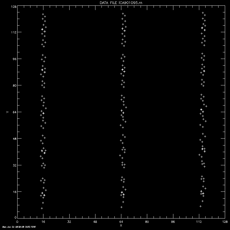
Figure 1: Simulated
images of 24 µm Focal Plane Survey Coarse.
Array Data Desired:
24 µm
Data Reformatting Option:
- Normal - One FITS multi-image extension file per AOR. (Output from MIPS DATPACK, one DCE in each image extension.
Task Dependencies
The telescope must be focussed. The Spacecraft must be pointing and tracking optimally. The PCS, PCRS, and IRU must be calibrated. The 24 um array and scan mirror must be fully operational. The 24 um photometry AOT must be validated.
- MIPS-121: 24 µm focus
- MIPS-910: 24 µm darks
- MIPS-917: 24 µm flat
- IPF run is to occur after FTU#8 (PAC filer and OET CTA Frame Tool inputs)
Calibration Dependencies
Calibration products needed:
- 24 µm flats
- 24 µm darks
- Items needed by IPF team for this task to run with the IPF filter software:
- IPF team Labeling convention for files: XXYYYZZZ.m where,
- XX for type of file (example FF for Offset file, IF for output data, CS for Centroid supplemental file)
- YYY for the version number, '001' to '499' for Coarse survey, '501' to '999' for Fine Surveys
- ZZZ for the Frame table number associated with the Prime Frame being calibrated. Use 095 for the 24 µm array. .
- CB file: The OET Centroid File and Generation Tool is run to generate a
centroid B file (CB file)
- A and As files: SIST generates a A and AS files (attitude history files)
and emails them to IPF team.
- FF file: The MIPS team generates an Offset file (match derived frames
to prime frames) and ftps to IPF team (this can be done before launch and has been).
- CS file: The MIPS team generated a CS file (Centroid supplemental file) to
IPF team. This can be done before launch and has been.
Output and Deliverable Products
- Output of MIPS DAT:
A calibrated data file with appropriated header keywords.
The name of this file will be "mips_YYY095.fits", where
where "YYY" is 3-digit string denoting run number, and "095" is
IPF code for 24 µm data.
This file is sent to B. Wheaton's centroiding program.
- Output from Centroid program:
A centroided data file.
The calibrated data is centroided and the centroided
data filename is CAYYY095.m, where the YYY is the version number. This file is
sent to the IPF team.
- Output from IPF team which the MIPS team analyzes:
- IF file: output data from a single IPF run.
- MF file: output data from a multi-run IPF run
- The FF file (offset file) and CS file (centroid supplemental file) have
been generated and sent to the IPF team. Unless the results from the coarse survey
result in significant changes to these files, these files will not be changed
for the fine survey.
Data Analysis
Task 130 is run both in Campaign F and Campaign G. The results from
both runs are used to update Frame Table # 9.
Data Analysis Campaign F:
- JPL MIPL transfers downlink data to SSC.
- SSC downlink ops processes data and places results in sandbox.
- SSC MIPS IST uses FTZ to transfer AOR data
from sandbox to SSCIST21. The data is run
through MIPS DATPACK routine which repackages the data to run with
the Arizona data analysis tool (DAT). The data are then calibrated
using the Arizona DAT package.
- MIPS DAT options.
- Run mips_sloper : with following options:
- mips_sloper -j dirname filename
- -j : directory below $MIPS_DIR/Cal to find calibration files.
- For 24 micron array - dark is applied at sloper level. Use -b: not to do the 24 micron dark subtraction.
- Run mips_caler : with following options:
- mips_caler -F flatfield_filename -C pathname
- -C path is the path to where the calibration files live. If you do not use
the _C then the default will be used.
- -l (to turn off latent correction) filename
- if you want to apply the latent correction then do not do -l and
use -L filename (text file with Si latent correction coefficients)
- The calibrated data file mipsfps_YYY095.fits
(YYY a 3-digit integer string, identifying the run number) is a
FITS multi-extension image file, one extension per DCE.
- Run Xsloper_view and check to make sure data seems reasonable.
- The calibrated data file is placed in sscist21:
/mipsdata/fps/inpdat. File is linked to processing subdirectory
(currently /home/sscmip/users/waw/fps).
- The MIPS IDL Centroid File Generation tool, mipspos.pro,
is run according to detailed instructions in
sscist21: /home/sscmip/users/waw/fps/fps.doc. This program
generates a set of PSF files for the centroiding program, as a function of
source (X,Y) on array and CSMM position using STINYTIM.
- The centroided output files CAYYY095.m (and CSYYY095.m just passed along)
are placed on the TFS at SSC and transfered to DOM at JPL.
- IPF team retrieves previously approved spreadsheet
and SSC's CA/CS files from DOM.
- IPF filter is run using input files: CB,A,AS,O, CA, CS files and the
previously approved spreadsheet.
- The output files (IF files) are placed on the DOM for MIPS team to analyze.
- End of Campaign F.
Data Analysis for Campaign G:
- The entire process (described in Campaign F) is repeated for Campaign G.
Analysis of output from Campaign F and Campaign G
- Results from the IPF filter for Campaign F and Campaign G
are analyzed by the MIPS team and compared to one another for consistency.
- On approval of consistency, the IPF team runs the IPF multi-run tool
and produces an output file, MF, that is placed on the DOM.
- THe MIPS IT/IST team retreives the multi-run results and reviews them.
Software Requirements
- STINYTIM for PSF generation.
- SSC downlink system.
- MIPS DAT
- IDL for IDL star centroiding program)mipspos.pro
- At JPL, IPF Filter program.
Actions Following Analysis
- After each run 130-F and 130-G the MIPS team recieves the results from
the IPF team and reviews them.
- After this this task has been run in both campaign F and campaign G
the MIPS team receives a MF file from the multi-run tool (produced by the IPF team).
The MIPS team reviews the MF file and approves or disapproves.
- When approved, SSC generates mini-spreadsheet for review and approval
by MCCB, followed by handoff to JPL OET, and uplink of FTU #9.
Failure Modes and Responses
- Failure of one campaign (F or G) to produce useful data
- If one of the runs looks bad, then go back and analyze the data better.
We may need to plot the data to look for bad data, we may need to edit the
CA file and resend it to the IPF team.
- We might need to ask the IPF team to look closer at their analysis.
- If one set is bad and can not be fixed, then use data from other campaign, if data appear reasonable and change
is not large?
- Results of F & G inconsistent, neither obviously bad, then average the results.
- Both results are bad - then reschedule observations.
Additional Notes