70µm WF Focal Plane Survey, Coarse

Principal: Jocelyn Keene
Deputy: Jane Morrison, Bill Wheaton
Data Monkey(s): Jane Morrison, Bill Wheaton
Priority: Critical
Downlink Priority: Normal
Analysis Time: Campaign H: 2880 minutes, Campaign I 2880 minutes, Analysis of combining H an I : 120 minutes
Last Updated:


Objective

To measure the pixel locations (i.e. array orientation, scale,and distortion) as a function of scan mirror angle for the 70 µm wide field array configuration.

Description

Use an IER based on the 70 µm photometry compact source AOT to measure the locations on the sky of several positions on the array as a function of scanning mirror angle.
This task is run in campaigns H and I. The data from each campaign is processed separately by the MIPS and IPF teams. The IPF team then combines the results from both campaigns. The results from the IPF multi-run are used to update Frame Table 10. The frame table updates for all the campaigns can be found in the following table:
Frame Table Updates

Data Collected

The observing strategy is similar to the 24 µm coarse. The IER collects 462 observations. The IER is set up so data is collected in 3 columns on the array: on the left-side, center and right-side of the array. After moving the telescope in the V direction according to the V offset, the observational patter is repeated 7 more times (with a V offset between each set).

Calibration Star

For the selected calibration star see the IER for this survey. The requirements on the 70 µm coarse focal plane calibration star are as follows:

  • In CVZ
  • Mips requirements: stellar brightness corresponding to S/N of 30 (3 sec integrations) 0.094 Jy, K mag 2.14

    Observing Strategy


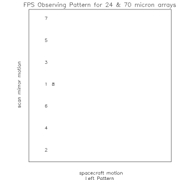
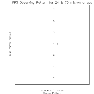
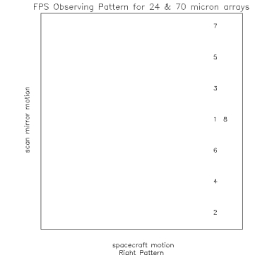
    Figure 1. Observing Pattern at 3 locations on the detector. Note size of box is not the total size of the array but a portion of the central region which depends on array and if it is a coarse or fine survey

    Definitions:

  • W axis direction is defined by the Frame Table, and is always within +/- 90 degrees of the TPF z axis as projected on the sky. Motion along this axis corresponds to motion in the spacecraft motion (left/right).
  • V axis direction is defined by the Frame Table, and is always within +/- 90 degrees of the TPF y axis as projected on the sky. Motion along this axis correspond to motion in the scan mirror direction (up/down).
  • W offset, the amount of motion in the W direction which results in the spacing between left array, middle array and right array observations
  • V offset, the amount of motion in the V direction which occurs between a set of observations.

    70 µm Coarse FPS observational parameters:

  • W offset = 120 arc seconds
  • V offset = 60 arc seconds
  • W dither = 15 arc seconds
  • V dither = 15 arc seconds
  • mirror locations for 1 position shown in figure 1.
    1. position 1 = 0
    2. position 2 = -60
    3. position 3 = 20
    4. position 4 = -40
    5. position 5 = 40
    6. position 6 = -20
    7. position 7 = 65
    8. position 8 = position 1 = 0

    Observational Strategy

  • Step 1
    1. PCRS observation
  • Step 2 - (total of 11 observations)
    1. Position the telescope so the data falls on the left side of array
    2. Position star at position 1 in figure 1 (left), turn stim on take an observation
    3. Turn stim off
    4. Take 8 DCES at positions shown in figure 1 (left)
    5. Position star at position 1, turn stim on and take observation
    6. With star still at position 1 turn stim off and take observation
    7. dither in V and W
    8. Repeat above 11 observations.
  • Step 3
    1. Move the space craft according to the W offset (120 arc seconds), image should now be on the center of the array.
    2. Position star at position 1 in figure 1 (middle), turn stim on take an observation
    3. Turn stim off
    4. Take 8 DCES at positions shown in figure 1 (middle)
    5. Position star at position 1, turn stim on and take observation
    6. With star still at position 1 turn stim off and take observation
    7. dither in V and W
    8. Repeat above 11 observations.
  • Step 4
    1. Move the space craft according to the W offset (138 arc seconds), image should now be on the right side of the array.
    2. Position star at position 1 in figure 1 (right), turn stim on take an observation
    3. Turn stim off
    4. Take 8 DCES at positions shown in figure 1 (right)
    5. Position star at position 1, turn stim on and take observation
    6. With star still at position 1 turn stim off and take observation
    7. dither in V and W
    8. Repeat above 11 observations in step.
  • Step 5
    1. PCRS observation
  • Step 6: move telescope according to V offset (60 arc seconds) and repeat steps 1-5
  • Step 7: move telescope according to V offset (60 arc seconds) and repeat steps 1-5
  • Step 8: move telescope according to V offset (60 arc seconds) and repeat steps 1-5
  • Step 8: move telescope according to V offset (60 arc seconds) and repeat steps 1-5
  • Step 9: move telescope according to V offset (60 arc seconds) and repeat steps 1-5
  • Step 10: move telescope according to V offset (60 arc seconds) and repeat steps 1-5

    Number of observations from step 1-5, 66. Step 1-5 repeated 7 times for a total of (66 * 7) = 462 observations.


    Data Reformatting Requirements

    Array Data Desired:

    70 µm Wide

    Data Reformatting Option:


    Task Dependencies


    Calibration Dependencies


    Output and Deliverable Products

    1. Output of MIPS DAT: calibrated data file with appropriated header keywords. The name of this file will be "mips_YYY107.fits", where where "YYY" is 3-digit string denoting run number, and "107" is IPF code for 70 µm WF array. This file is sent to B. Wheaton's centroiding program.
    2. Output from Centroid program: Centroid data file. The calibrated data is centroided and the centroided data filename is CAYYY107.m, where the YYY is the version number. This file is sent to the IPF team.
    3. Output from IPF team which the MIPS team analyzes:
      • IF file: output data from a single IPF run.
      • MF file: output data from a multi-run IPF run
    4. The FF file (offset file) and CS file (centroid supplemental file) have been generated and sent to the IPF team. Unless the results from the coarse survey result in significant changes to these files, these files will not be changed for the fine survey.

    Data Analysis

    Task 132 is run both in Campaign H and Campaign I. The results from both runs are used to update Frame Table # 10.
  • Process data for Campaign H:
    1. JPL MIPL transfers downlink data to SSC.
    2. SSC downlink ops processes data and places results in sandbox.
    3. SSC MIPS IST uses FTZ to transfer data from sandbox to SSCIST21.
    4. Data is repackaged with MIPS DATPACK
    5. The data are calibrated using the MIPS DAT using the following options
      1. Run mips_sloper : with following options:
        • mips_sloper filename
        • IF we do not use the default directory for the calibration files. Then use the -j option.
        • -j dirname : directory below $MIPS_DIR/Cal to find calibration files.
      2. Run mips_caler : with following options:
        • mips_caler -I illumination_correction_filename -D dark_filename-C pathname
        • -C path is the path to where the calibration files live. If you do not use the -C then the default will be used.
        • -D dark filename.
        • -I illumnation correction filename
      3. The calibrated data file mipsfps_YYY107.fits (YYY a 3-digit integer string, identifying the run number) is a FITS multi-extension image file, one extension per DCE.
      4. Run Xsloper_view and check to make sure data seems reasonable:
    6. The calibrated data file mipsfps_YYY107.fits is placed on sscist21: /mipsdata/fps/inpdat. File is linked to processing subdirectory (currently sscist21: /home/sscmip/users/waw/fps).
    7. The MIPS IDL Centroid File Generation tool, mipspos.pro, is run according to detailed instructions in sscist21: /home/sscmip/users/waw/fps/fps.doc.
    8. The output files CAYYY107.m (and CSYYY107.m - just passed along) are placed on the TFS at SSC and transfered to DOM at JPL.
    9. IPF team retrieves previously approved spreadsheet and SSC's CA/CS files from DOM.
    10. IPF filter is run using input files: CB,A,AS,O, CA, CS files and the previously approved spreadsheet.
    11. The IPF output files (IF files) are placed on the DOM for MIPS team to analyze.
    12. End of Campaign H.
  • The entire process above is repeated for Campaign I.
  • Results from the IPF filter for Campaign H and Campaign I are analyzed by the MIPS team and compared to one another for consistency.
  • On approval of consistency, the IPF team runs the IPF multi-run tool and produces an output file, MF, that is placed on the DOM.

    Software Requirements


    Actions Following Analysis


    Failure Modes and Responses

    1. Failure of one campaign (H or I) to produce useful data
      • If one of the runs looks bad, then go back and analyze the data better. We may need to plot the data to look for bad data, we may need to edit the CA file and resend it to the IPF team.
      • We might need to ask the IPF team to look closer at their analysis.
      • If one set is bad and can not be fixed, then use data from other campaign, if data appear reasonable and change is not large.
    2. Results of H & I inconsistent, neither obviously bad, then average the results.
    3. Both results are bad - then reschedule observations.

    Additional Notes