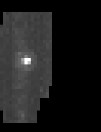
Figure 1: 70/160µm images of Ampella.
Principal:
Deputy:
Analyst:
AORKEYS:
Last Updated:
All data were processed with version 2.62 of the DAT, turning off the electronic nonlinearity correction and using the flight calibration files. The 70µm and 160µm data were processed as described in the mips-922 and mips-924 writeups, respectively.
Figure 1: 70/160µm images of Ampella.
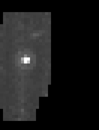
Figure 2: 70/160µm images of Beatrix.
Figure 3: 70/160µm images of Tercidina. Note that the
160µm image is flipped in both axes relative to the other images here.
The calibration factor (in units of µJy/arcsec²/(MIPS160Unit)) was calculated from three sources, as follows: The 70µm observations were reduced and calibrated using the standard calibration factor (1.49×10⁴ µJy/arcsec2/MIPS70Unit). The results were divided by a color correction appropriate to the temperature of the source (assumed to be 250 K for all sources). This quantity for each target is the one labeled "Measured 70µm Flux" in the table below. The results were then scaled to 160µm using a flux ratio derived from the same model which produced the flux predictions. These results were then multiplied by the appropriate color correction factor to put them back on the 10,000K blackbody scale used by the other bands. This quantity for each target is referred to as the "transfer" prediction in the table below. These predictions were then compared to the measured counts to determine the calibration factor. Conversion between surface brightness and integrated flux units were done assuming a pixel scale of 9.89 arcsec. at 70µm and 16.0 arcsec. at 160µm.
The results are summarized in the following table:
|
Photometry |
||||||||
| Target | Predicted 70µm Flux (Model) | Predicted 160µm Flux (Model) | Predicted 70/160µm Flux Ratio | Measured 70µm Data | Measured 70µm Flux | Predicted 160µm Flux (Transfer) | Measured 160µm Data | Calibration Factor |
| |
(Jy) | (Jy) | |
(MIPS70Unit) | (Jy) | (Jy) | (MIPS160Unit) | (µJy/arcsec²/MIPS160Unit) |
| Ampella | 2.107±0.260 | 0.599±0.054 | 3.51±0.11 | 1.7440±0.0386 | 2.62±0.058 | 0.741±0.029 | 1.8593±0.1655 | 1557±151 |
| Beatrix | 2.307±0.327 | 0.667±0.071 | 3.45±0.13 | 2.0207±0.0320 | 3.04±0.062 | 0.875±0.038 | 3.6821±0.2733 | 928±79.8 |
| Tercidina | 3.909±0.516 | 1.108±0.109 | 3.52±0.13 | 2.6991±0.0508 | 4.06±0.076 | 1.145±0.048 | 4.1705±0.2720 | 1072±83.1 |
A straight average of the results gives a calibration factor of 1186±63.3µJy/arcsec²/(MIPS160Unit). A weighted average that includes all the asteroid data obtained so far is 1156±42.5µJy/arcsec²/(MIPS160Unit). A plot of all the asteroid data is shown in Figure 4.
Figure 4: 160µm calibration factors
vs. flux, from campaigns 2 and 3.
The calibration factor at 160µm was calculated by transferring the 70µm calibration to 160µm via asteroids observed in common.
none