OSMOS Long-slit Data Reduction
Before We Begin
This page is designed to walk you through reducing long-slit data with the OSMOS instrument, as well as the MDM4k chip, on the MDM 2.4m Hiltner telescope using standard IRAF procedures. I am going to assume that you have followed along with my guide for using OSMOS here, and have taken the following images, described below.
We're going to run the reduction sequence on some sample data from January of 2015. You can download a big file that has all of the data I'm going to be reducing here.
When I reduce data, I copy everything into a separate folder from where the raw data is stored. It's pretty important that you never just edit or reduce raw data, as you may want to start from scratch. Actually, you will want to start from scratch, since this process is complicated, and often you'll want to go back and see how changing one step affects the final data. At the same time, it's good to keep the raw data in a place where it's easily shareable with others.
The object we'll be looking at is the galaxy SDSS J0911+6152. which is at a redshift of z = 0.027. At this redshift, since we'll be reducing an optical spectrum, we are focusing on the spectral range that includes both the [OIII]5007 and H-alpha emission line complexes. You can see an example of the SDSS spectrum for this object, which you can compare to your final product.
Before we begin, let's take a look at the data that was taken:
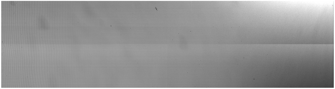
1. DarksBecause our science targets were observed with 1800s exposures, we took a series of 1800s dark images. We also took darks with the exposure times corresponding to the flats and arcs. Just to be complete, I will discuss the procedure for dark reduction of OSMOS data, but it turns out, OSMOS does not have a huge amount of dark current to speak of, so you probably won't need to dark reduce your data.
2. Flats
We took twilight sky flats, with the slit and disperser in, in order to get an image of how the slit and disperser illuminate the chip. We also took dome flats, where we pointed the dome at a screen during the day, and these are a good alternative to twilight flats. However, both the twilight and dome flats have sky features, which make them unsuitable for using for flat fielding. So, we also took instrument ("MIS") calibration flats, but the illumination pattern is not ideal, so we'll have to use the sky flats or the dome flats to correct. I walk through this process in this step.
3. Arcs
Based on the slit that we're using, we used Argon arcs, with 300s exposures. You can read the OSMOS wavelength calibration recommendations here. In the folder of sample data, I've included the file "osmos_Argon.dat", and the pdf "osmos_argon_12inner.pdf" which will be important for calibrating the wavelength. Both these files, as well as files corresponding to other slit configurations for OSMOS are downloadable from the above linked site.
4. Science Data
We took three 1800s exposures for our target. We took three images in order to remove cosmic rays using a median combining.
5. Biases
Because we are using the MDMD4k chip, we can use an overscan region to remove the bias from each of the quadrants. If we were using another chip, we'd have to take bias images, and subtract them.
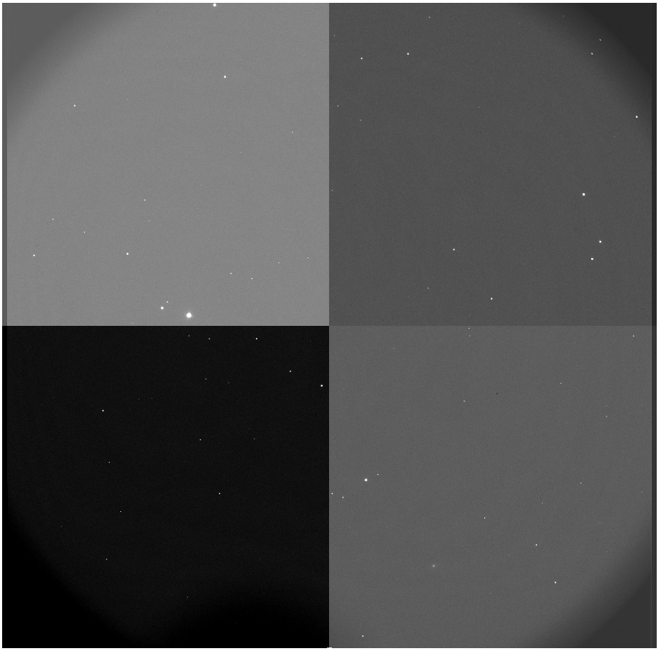
Removing The Bias
So, the MDM4K has four chips, all with different bias levels. You can put an overscan region around the edge of the chip, and I'm going to be using an X overscan region of 32 pixels:
  OVERSCNX=      32 /
  OVERSCNY=      0 /
If you are using a Y overscan region, you'll have to modify the procedure accordingly. I've written a perl script that subtracts the bias from MDM4K data called bias_4k.pl. If you prefer pyraf, Paul Martini has also written a bias reduction script (bias4k.cl). I'll walk through how both scripts work using a file called "j0911.1074.fits". First:
  > colbias j0911.1074.fits j0911.1074.1.fits bias=[1:32,1:2032] trim=[33:2064,1:2032] median- interac- function="legendre" order=4
  > colbias j0911.1074.fits j0911.1074.2.fits bias=[1:32,2033:4064] trim=[33:2064,2033:4064] median- interac- function="legendre" order=4
  > colbias j0911.1074.fits j0911.1074.3.fits bias=[4097:4128,1:2032] trim=[2065:4096,1:2032] median- interac- function="legendre" order=4
  > colbias j0911.1074.fits j0911.1074.4.fits bias=[4097:4128,2033:4064] trim=[2065:4096,2033:4064] median- interac- function="legendre" order=4
This IRAF procedure will look through a region of the image specified by the bias keyword in the input line, and then it will calculate the median level in this region and subtract it from the region specified by the trim keyword. These four lines split the MDM4K image into four bias-subtracted images, which will have to be pasted together. Notice the regions specified correspond to the edges with the overscan.
> imarith j0911.1074.fits[33:4096,1:4064] * 1.0 j0911.1074.trim.fits ver-
We want to paste the various quadrants into an image of the correct size, so we'll first create a trimmed science image, where we cut out the bias portion. We're going to paste the bias subtracted images over this image.
  > imcopy j0911.1074.1.fits[1:2032,1:2032] j0911.1074.trim.fits[1:2032,1:2032] ver-
  > imcopy j0911.1074.2.fits[1:2032,1:2032] j0911.1074.trim.fits[1:2032,2033:4064] ver-
  > imcopy j0911.1074.3.fits[1:2032,1:2032] j0911.1074.trim.fits[2033:4064,1:2032] ver-
  > imcopy j0911.1074.4.fits[1:2032,1:2032] j0911.1074.trim.fits[2033:4064,2033:4064] ver-
And now we use imcopy to paste the quadrants into the correct regions of the trimmed image that we just made.
  > imdel j0911.1074.1.fits
  > imdel j0911.1074.2.fits
  > imdel j0911.1074.3.fits
  > imdel j0911.1074.4.fits
  > rename j0911.1074.trim.fits j0911.1074.b.fits
And finally, we'll delete the individual quadrant images. We also rename our final file to the filename with a b.fits on the end. Throughout this guide, I use my file naming convention where I append a series of letters onto the end of the file name to indicate that I've done certain steps.
At this point the script adds information to the header to indicate you've run bias subtraction:
  > hedit j0911.1074.b.fits OVERSCAN "[1:32,*] and [4097:4128,*]" add+ del- ver- show- upd+
  > hedit j0911.1074.b.fits CCDSEC "[33:4096,1:4064]" add+ del- ver- show- upd+
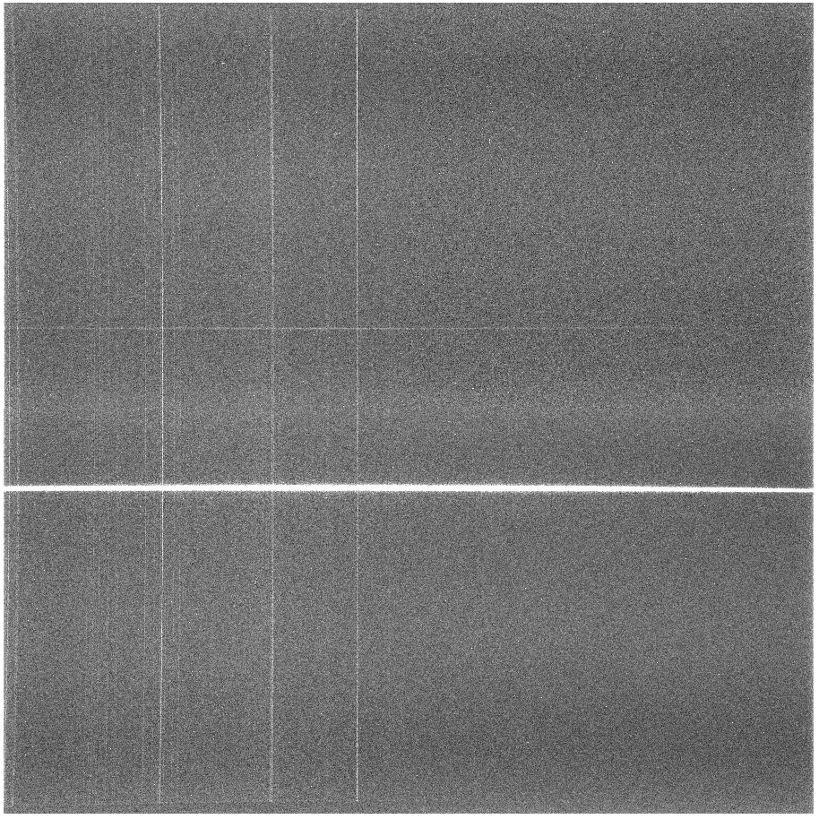
If everything has gone well, you can take the raw j0911.1074.fits and bias subtract it:
 -->
-->
If you want to use bias4k.pl, you should have IRAF installed, as the perl
script will call IRAF using the command cl. The script is
run in this way:
% perl bias_4k.pl j0911.1074.fits
And it just does everything as was just described! (NOTE: the little percent
sign in the code above means that this is executed from outside of IRAF, in
a terminal window.) You can include the .fits
extension or not, it's up to you. If you are wanting to take a frame that has been
binned, or only represents the central 1k portion of the chip, I have two other
version of the program. The script bias_1k.cl will work
on 1x1 binned data from the central 1k portion of the MDM4K chip. Also, the script
bias_4k_4x4.cl will work
on 4x4 binned data from the entire 4k MDM4K chip.
You are going to want to bias reduce all of the data that we are going to be using, and I'll try to remember to keep reminding you in this guide.
Creating The Master Flat
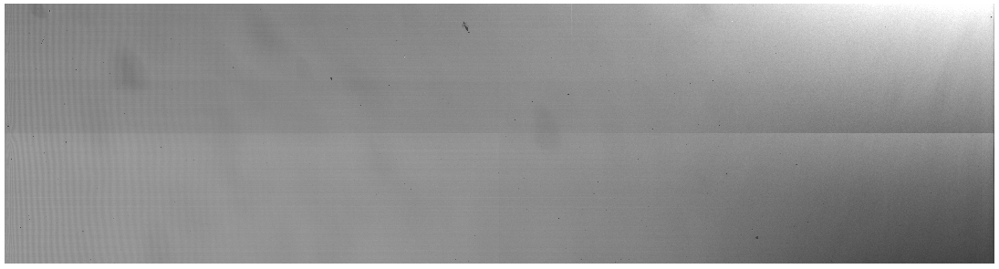
First, let's go and grab the various flats, and bias reduce them. Here are the flats we'll be using:
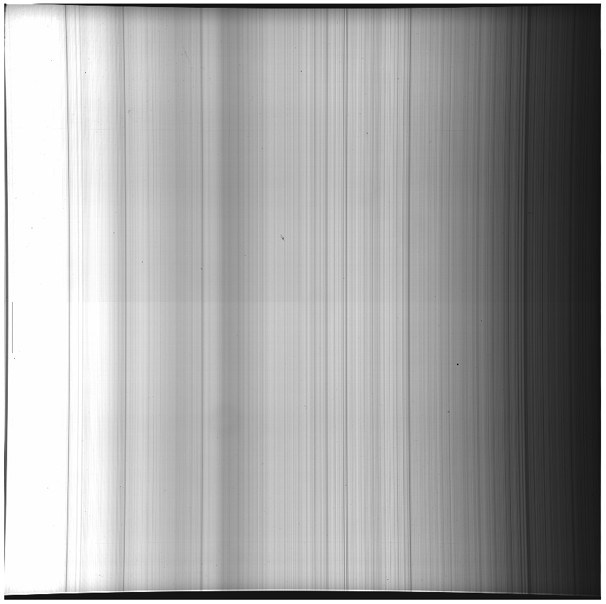
MIS Instrument Flats
instflat.4005.fits, instflat.4006.fits, instflat.4007.fits, instflat.4008.fits, instflat.4009.fits
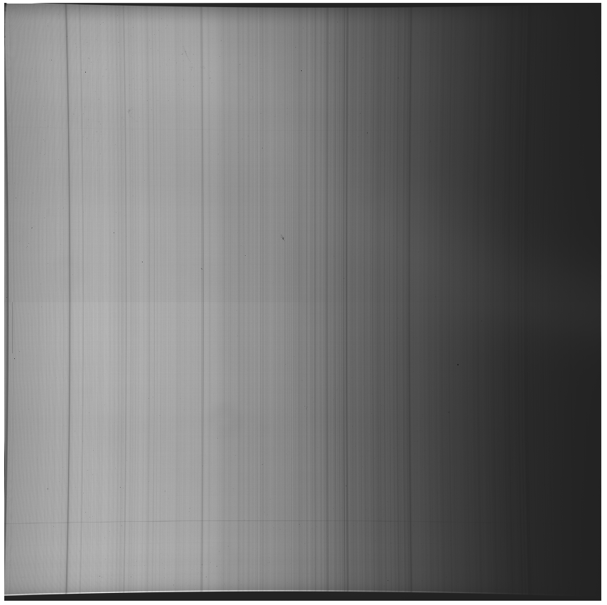
Twilight Flats
twiflat.1016.fits, twiflat.1017.fits, twiflat.1018.fits, twiflat.1019.fits
Dome Flats
domeflat.3004.fits, domeflat.3005.fits, domeflat.3006.fits
Here are some examples:
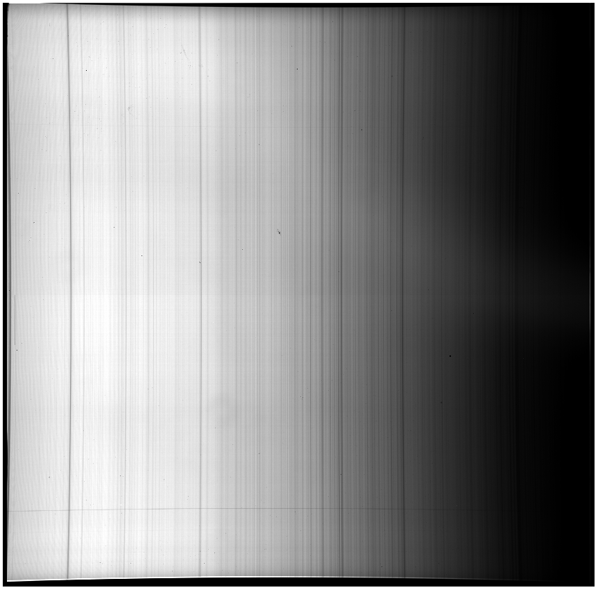
 Instrument Flat
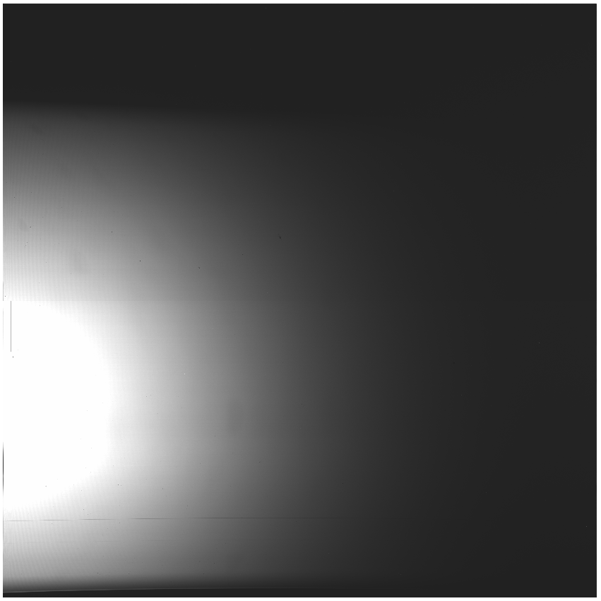
 Twilight Flat
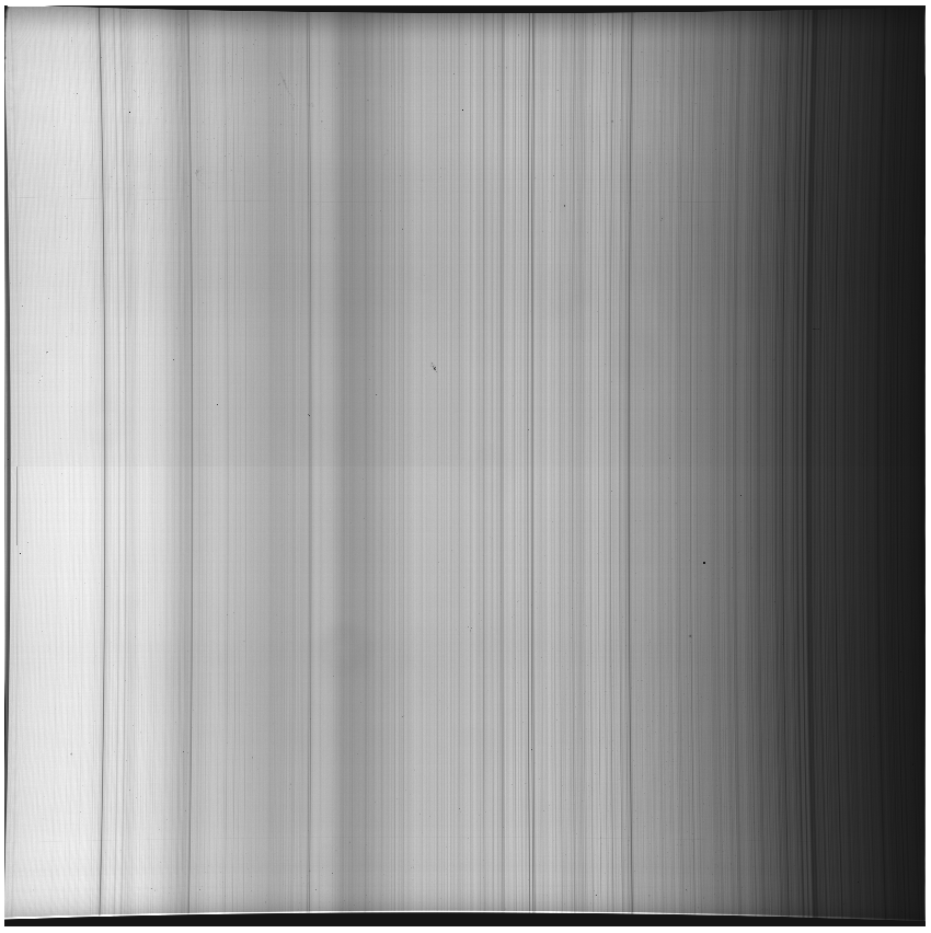
 Dome Flat
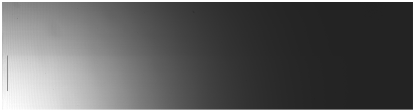
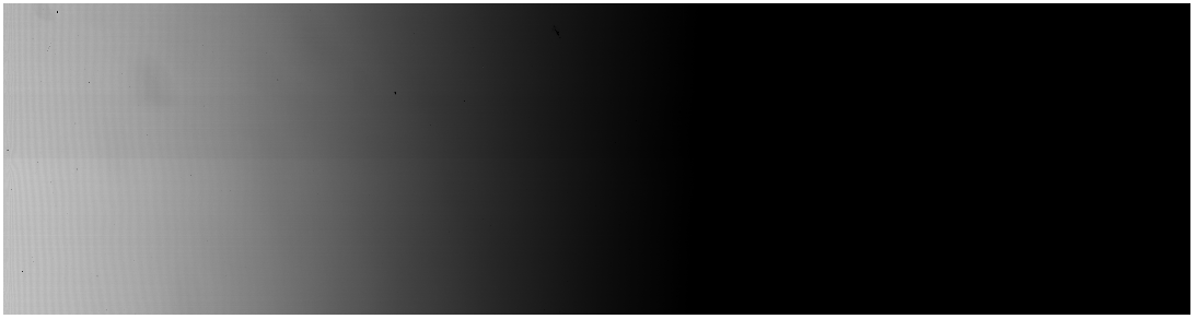
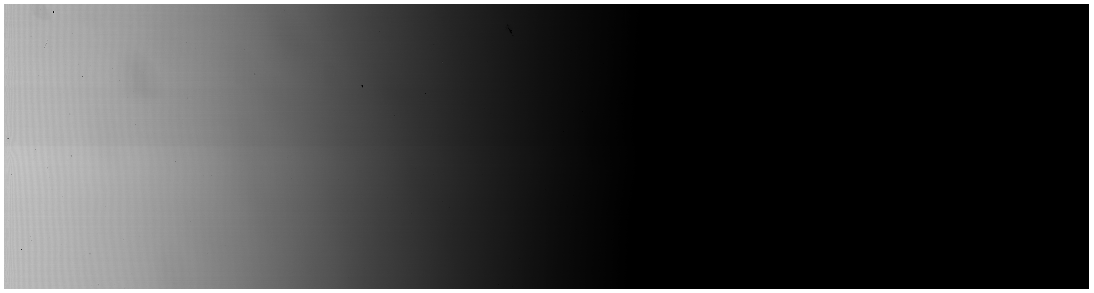
First, we'll need to run bias_4k.pl on each individual frame. You should look to see how the bias is running on the final images (example bias subtracted images: instrument flat, twilight flat, dome flat). You should hopefully not able to see the seams between the various quadrants.
% perl bias_4k.pl instflat.4005.fits
(etc., etc.)
Once you're happy with your bias subtraction, it's time to combine the individual flats (of a specific
type) to remove the cosmic rays. I usually put the file names into various lists
("skyflats.list", "domeflats.list", etc):
  % ls instflat*.b.fits > misflats.list
  % ls twiflat*.b.fits > skyflats.list
  % ls domeflat*.b.fits > domeflats.list
Then I'll run the IRAF task flatcombine to combine the flats. The
taks flatcombine can be found in the noao.imred.ccdred package,
and in IRAF, you just have to type the name of the package to open it. So, here,
you'd type noao to open that package, then, imred
then ccdred. From here, we can combine the flats:
  > flatcombine @skyflats.list output=skyflatmed.b.fits combine=median reject=avsigclip process=yes scale=mode
  > flatcombine @misflats.list output=misflatavg.b.fits combine=average reject=avsigclip process=yes scale=mode
  > flatcombine @domeflats.list output=domeflatmed.b.fits combine=median reject=avsigclip process=yes scale=mode
Note: If you are running things from a fresh install of IRAF, you might
run into an error where it says "No bad pixel mask found". To fix this, you
have to actually change some parameters that you'll want to change anyway,
in a secret package that flatcombine is using called ccdproc,
and it's found in noao.imred.ccdred:
> epar ccdproc
Make sure that these parameters are all set to "no":
  (fixpix =                   no) Fix bad CCD lines and columns?
  (oversca=                   no) Apply overscan strip correction?
  (trim   =                   no) Trim the image?
  (zerocor=                   no) Apply zero level correction?
  (darkcor=                   no) Apply dark count correction?
  (flatcor=                   no) Apply flat field correction?
  (illumco=                   no) Apply illumination correction?
  (fringec=                   no) Apply fringe correction?
  (readcor=                   no) Convert zero level image to readout correction?
  (scancor=                   no) Convert flat field image to scan correction?
(Remember, when you're done with a parameters file, type ctrl-d to
get back to the command line) If you're getting the error about the bad pixel mask, well, that's because
flatcombine is talking to ccdproc before it combines
the flats, and if fixpix = yes, then ccdproc will
look for a bad pixel mask to fix bad pixels in the images before combining them.
We haven't actually created a bad pixel mask, so ccdproc doesn't
need to do anything. Just set everything to "no" here and you should be fine.
Notice that when we run flatcombine we're using median combining for the sets where we have three
or more files. This will remove any cosmic rays, although this shouldn't be
much of an issue because the exposure times are pretty short. Now you should
have the bias-reduced combined flat frames (example combined frames: misflatavg.b.fits,
skyflatmed.b.fits,
domeflatmed.b.fits). We'll use these to create a master
spectral flat which we can use to to flatten our science images.
Side note: As I mentioned in the introduction, I am not going to be
dark subtracting these frames. You can go and take individual darks for
each of the exposure times for your flats, but for OSMOS+MDM4k, the dark
current is pretty negligible in these flats.
When I was on this observing run, I took the data in the full 4k by 4k mode
of OSMOS, even though most of our spectra were quite near the center of each
image. It's actually good to trim the flats for this process, since we don't
care about flat fielding away from where the various spectral traces lie.
As a result, I'm going to be trimming in the y-direction, but I'll keep the
full range (pixels 1 to 4064) in the x direction.
We can use imcopy to trim images:
  > imcopy skyflatmed.b.fits[1:4064,1500:2564] skyflatmed.b.trim.fits
  > imcopy misflatavg.b.fits[1:4064,1500:2564] misflatavg.b.trim.fits
  > imcopy domeflatmed.b.fits[1:4064,1500:2564] domeflatmed.b.trim.fits
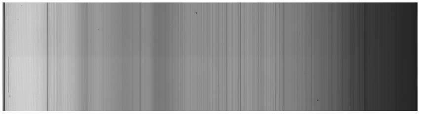
Take a look to see what we've done (example trimmed frames: misflatavg.b.trim.fits,
skyflatmed.b.trim.fits,
domeflatmed.b.trim.fits)
The next step is to use the IRAF task blkavg
to collapse our avg and median flats in the spatial direction. We are going to
do this so that we can utilize the sky flat or the dome flat to estimate the full illumination
pattern.
  > blkavg skyflatmed.b.trim.fits output=skyslitmed.b.trim.fits option=average b1=4064 b2=1
  > blkavg misflatavg.b.trim.fits output=misslitavg.b.trim.fits option=average b1=4064 b2=1
  > blkavg domeflatmed.b.trim.fits output=domeslitmed.b.trim.fits option=average b1=4064 b2=1
Notice that b1 is set to the width of the images, while b2 is 1, so this means we are going to keep the final image with height 4064, but with length 1 pixel. Since up and down on our images corresponds to the spatial direction, we have eliminated the "dispersion" or wavelength direction. So, I won't show examples of these files, since they're one pixel wide. Not too interesting.
Now, let's divide the skyslit and domeslit by the misslit, which will produce a quotient image that we can smooth and fit, and then multiply by the misflat to correct for the improper illumination.
  > imarith skyslitmed.b.trim / misslitavg.b.trim quotient.1.fits
  > imarith domeslitmed.b.trim / misslitavg.b.trim quotient.2.fits
And now we're going to run fit1d to fit this quotient, which will allow us
to smooth over the sky lines. Notice we're running this noninteractively,
since we trust that things shouldn't be too bad with a 4th order polynomial.
If you don't trust it, take a look at the final output using implot.
  > fit1d quotient.1 smoothedquotient.1 type=fit interactive=no function=spline3 order=4 low_reject=3.0 high_reject=3.0 niterate=1 naverage=1
  > fit1d quotient.2 smoothedquotient.2 type=fit interactive=no function=spline3 order=4 low_reject=3.0 high_reject=3.0 niterate=1 naverage=1
The next step is to expand the smoothed quotient file to the size of the
trimmed image, and we'll use the IRAF task blkrep:
  > blkrep smoothedquotient.1 output=skybalance.1.fits b1=4064 b2=1
  > blkrep smoothedquotient.2 output=skybalance.2.fits b1=4064 b2=1
And, then, we'll multiply the misflat by our
new skybalance files to correct for the illumination, using imarith:
  > imarith misflatavg.b.trim.fits * skybalance.1.fits flatbalanced.1.fits
  > imarith misflatavg.b.trim.fits * skybalance.2.fits flatbalanced.2.fits
You can see what flatbalanced.1.fits and flatbalanced2.fits look like by
clicking those links. Finally, let's run the IRAF task response,
which is found in the noao.twodspec.longslit packages. We'll use
response to create the normalized response corrected flat. You should have noticed that
I'm creating two of these, one using the twilight flat and one for the dome flat,
so you can determine which flat looks better in the end:
  > longslit.dispaxis = 1
  > response flatbalanced.1.fits flatbalanced.1.fits flatnorm.1.fits interactive=no threshold=INDEF sample='*' function=spline3 order=30 low_reject=3.0 high_reject=3.0 niterate=1 grow=0.0
  > response flatbalanced.2.fits flatbalanced.2.fits flatnorm.2.fits interactive=no threshold=INDEF sample='*' function=spline3 order=30 low_reject=3.0 high_reject=3.0 niterate=1 grow=0.0
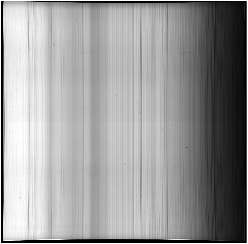
Here are what both of these flats look like:
Flatnorm.1.fits (made from the twilight flat):
Flatnorm.2.fits (made from the dome flat):
Notice, both of them look really good. For the purposes of this reduction, we'll be going with flatnorm.1.fits, which was made using the twilight flats.
Make The Dark Image (Optional!)
Again, users of OSMOS and the MDM4k chip shouldn't feel the need to create a dark image for the science data, but in case you want to remove the dark current, we can create a dark frame. We took a series of 1800s dark frames, which are included in the folder. These are images dark.0006 through dark.0010. I keep them in a folder called "dark", but you can do what you want. We'll start by bias subtracting these frames:
  % perl bias_4k.pl dark.0007.fits
  % perl bias_4k.pl dark.0008.fits
  % perl bias_4k.pl dark.0009.fits
Next, you'll want to combine these bias subtracted dark frames:
  > ls *.b.fits > dark.list
  > imcombine @dark.list dark_combine.fits combine=average reject=minmax nhigh=1 nlow=1 zero="none" sigma="sig_dark.fits" scale=exposure weight=none
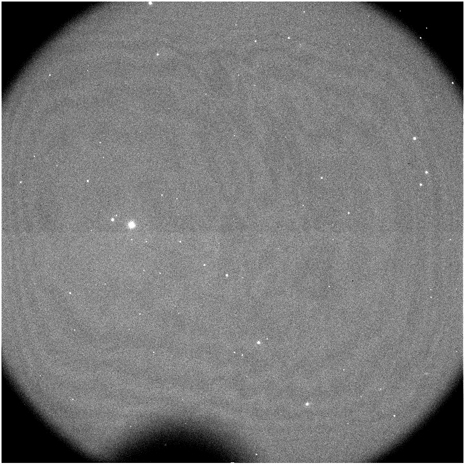
Take a look at this exposure. In mine, the dark current for an 1800s exposure is pretty negligible:
We can subtract this from our science exposures if we want, but it's not going to change things appreciably.
Prepare the Arc Image
We are going to start the process of wavelength calibration by bias subtracting the arc image.
% perl bias_4k.pl arc.2079.fits
 -->
-->

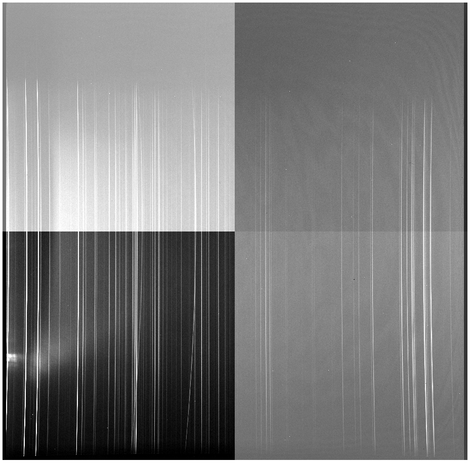
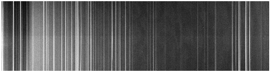
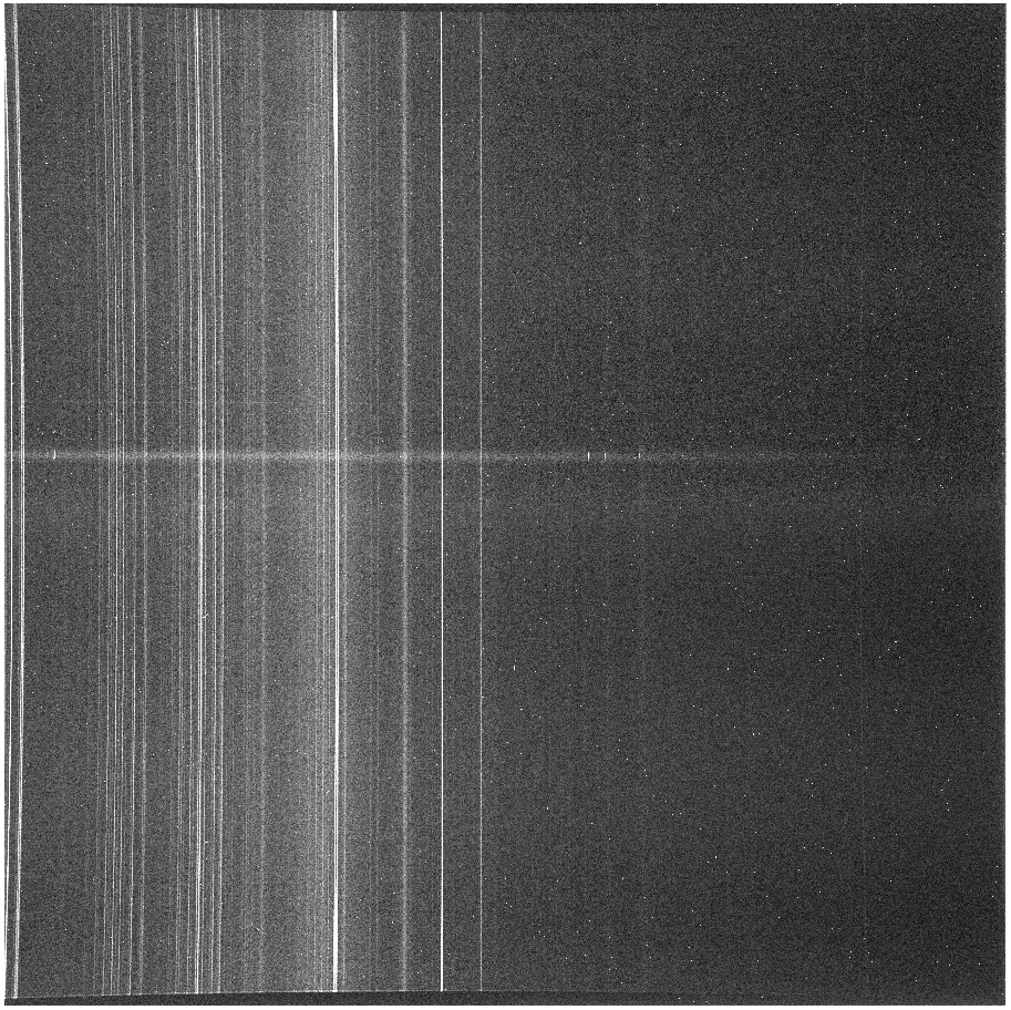
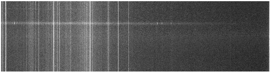
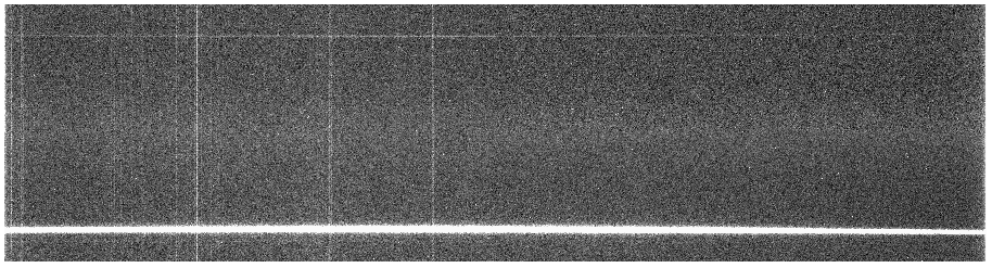
Now that we've bias subtracted the arc, we can go and just trim:
> imcopy arc.2079.b.fits[1:4064,1500:2564] arc.2079.b.trim.fits
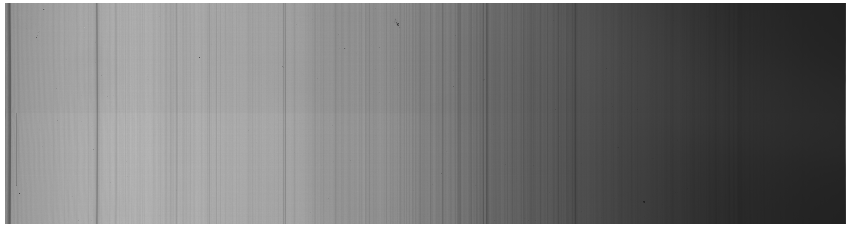
We don't divide by a flat, or dark subtract these images, because all we care about is the position of the emission lines, which are easily seen in the resulting image:
Identify
So, now we're going to do a pretty complicated portion of this reduction
procedure, the part where we identify emission lines in the arc lamp spectrum for
the purposes of wavelength calibration. The way in which this works is that
we use an IRAF task called identify, which is found in the noao.onedspec
package. This procedure plots the center of the arc image, showing the peaks, and then allows the
user to provide the wavelengths of those peaks. From here, a fit will be performed
between the pixel values and the wavelength values for the peaks near the center
of the image, and you will move on to the task reidentify.
For this redshift and grating configuration, we've used an Argon arc lamp. For the purposes of running identify, we're going to want to download the file osmos_Xenon.dat (which is included in the sample data) to the location where we're reducing this data. A whole bunch of line lists are found here. With this file downloaded, we'll also probably want some sort of image of the optical Argon spectrum to compare to. For this configuration, you can find this in this pdf (again, this is included). On the OSMOS wavelength calibration page, you can find the corresponding pdfs for the other lamps and instrument set-ups.
Anyway, let's run identify on the arc image:
> identify images=arc.2079.b.trim.fits coordlist=osmos_Argon.dat function=chebyshev section="middle line" order=5 fwidth=6. cradius=6
There are a few important things to notice:
First, we need to make sure that the coordlist is set to the file that you should have downloaded corresponding
to that particular arc lamp. It's a pain to input the exact-to-the-decimal wavelength
value for each and every line you want to fit, so a coordlist is used. When you
input a wavelength value, identify will go
through the coordinates list and grab the nearest wavelength in the list, which
makes everyone's lives easier. Also, once you input a few correct wavelength values
and create a rough fit, identify can be told to
look through the coordlist and just find the peaks that are closest in rough
wavelength to the lines in the list, which speeds things up considerably.
Secondly, the order for the fit specified here is 5, but you want to go
with the lowest order that produces results you think look
good. For some arc spectra, you may have to use order=3 or else
reidentify breaks as such a high order fit ends
up not being well constrained. It's not a huge deal in the grand scheme of
things, but do what you want.
Third, you're going to want to use section="middle line" since our
dispersion direction is right to left. Otherwise, we'd use section="middle column",
and identify would use the central column of the image for the
wavelength solution.
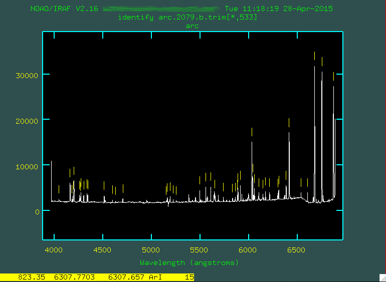
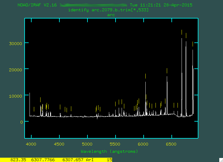
Now, when you run that identify line, you'll
be presented with the spectrum of the emission features from the center of the
image.
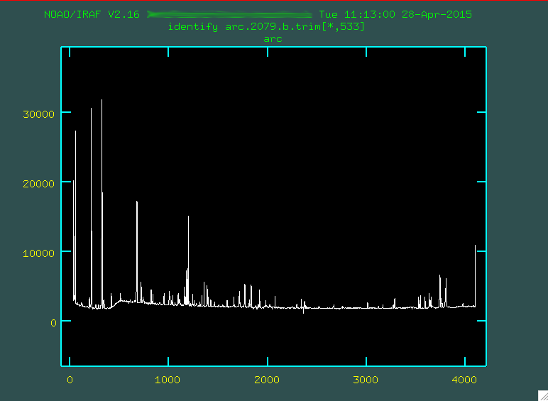
Each one of the spikes corresponds to an Argon emission line at a particular
wavelength, given in the pdf osmos_argon_12inner.pdf. Your job is to go
through and identify the lines you see in your sample arc
spectrum in the one you've measured here, and mark them. It's a little annoying
to try to do this from the zoomed-out image, so you can zoom in by moving the cursor
to the bottom-left of where you want to zoom, and typing w (for "window")
then e (for "edge, maybe?). Then you move the cursor to the top right
of where you want to zoom, and again type e again.
Here's an example focusing on the region from 0 - 500.
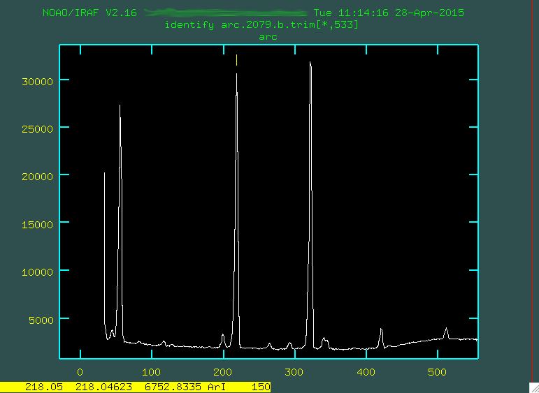
Notice in that image that the feature to the right of the number 200 is marked with a little yellow line. I went and found what line that was on the pdf (in this case, it was 6752.8335 Angstroms), and I moved the cursor over the line, typed
m, and then typed in the wavelength 6752.8335 and
pressed enter. This caused the line to be marked. If you make any mistakes,
you can always hover over the marked line and type d to delete it. Notice that the spectrum is
backwards from what is seen in the pdf of the lines. This is because, for OSMOS and the MDM4k
chip, the wavelength range has blue light on the right, red on the left.
To get out of a zoomed in window, you can type w then n
and w then m. By zooming, and looking at the pdf of
the actual emission lines, I marked some of the brighter lines:
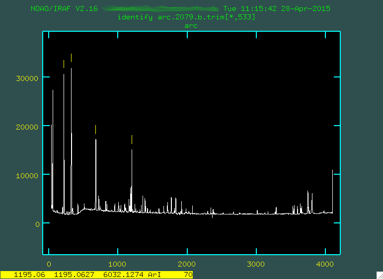
It's important to mark just enough lines to span the entire wavelength range, so you constrain the eventual fit across the whole chip. Here are the emission lines that I ended up going with to just start off with:

You want to make sure that the coordinates list you downloaded is in
the folder where you're running identify, or else it won't be able to
figure out which lines you are typing in. When you're happy with the number of
lines you've input, press f to fit a polynomial to these
individual points.
Ignore how this fit looks, because it's trying to fit a polynomial to
just a few points. Press q to go back to the spectrum,
and press l to have the program automatically find lines from the coordlist, using
the first pass fitting you just ran.
Now, press f to fit all of these new lines.
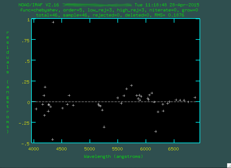
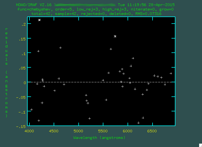
The fit looks ok, but you might have to go through and trim out some emission lines that were either poorly fit, or incorrectly identified. To do this, line the cursor up over these points and press
d to delete
these points. Here are the points I didn't like:
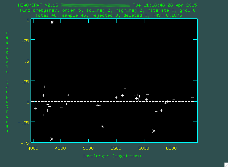
Whenever you want, you can press
f to re-fit. Watch the rms, which
measures the goodness of fit. If you press q and then f again,
you'll only see the lines being fitted.
You may want to change the order of the fit, too, by typing
or: X,
where X is the number of the order, so for instance, or: 6
would give a 6th order fit.
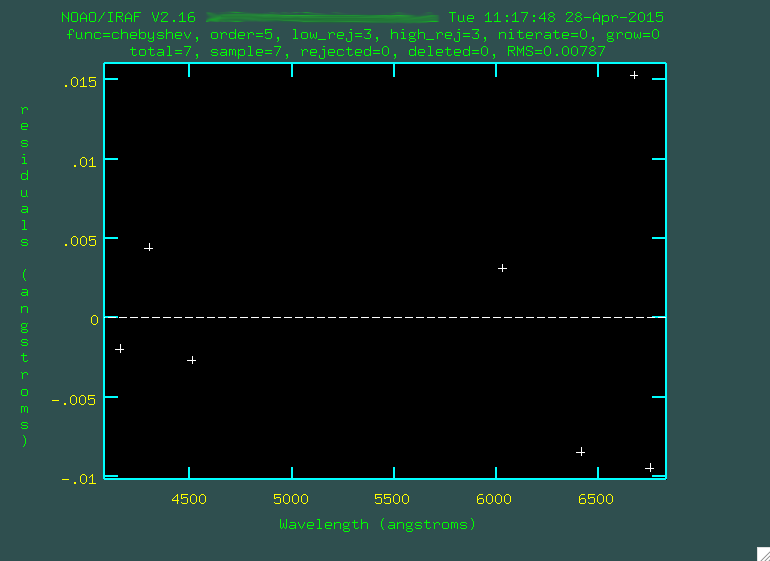
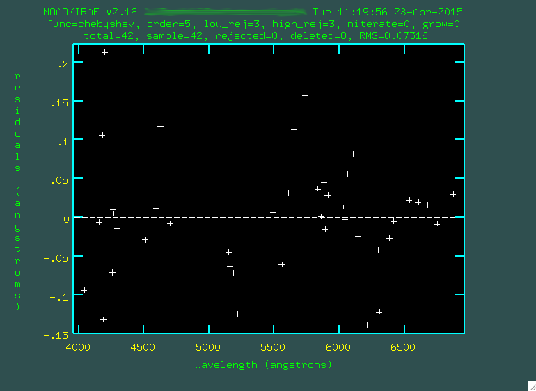
I went through and trimmed out a few more points:
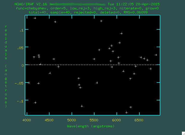
Look at that rms drop!
Eventually, I was happy with the fit, and once you're happy, you can press q on the page
with the spectrum, and the IRAF window will ask you if you want to write the feastures to the
database. Choose "yes." If there is no database folder present in the folder where
you're doing the reduction, a folder will be created, and a file will be put there
(in our case, the file is called idarc.2079.b.trim) that has the
parameters from this fitting.
Reidentify
reidentify
is now going to go through every row in the image and re-run
identify using the initial guess fitting you
just created, and effectively trace the curvature of the lines in the spatial
direction. It's run in this way:
> reidentify reference=arc.2079.b.trim.fits images=arc.2079.b.trim.fits section="middle line" interactive=no newaps=yes override=no refit=yes nlost=20 coordlist=osmos_Argon.dat verbose=yes > reidentify.log
Note that this is run non-interactively, which is fine. The reference image
is the same as the image we are working on. So, this will spit out the resulting
lines from the individual runs of identify into a file called "reidentify.log":
  REIDENTIFY: NOAO/IRAF V2.16 yourusername@yourcomputer Tue 11:25:58 28-Apr-2015
  Reference image = arc.2079.b.trim.fits, New image = arc.2079.b.trim, Refit = yes
           Image Data    Found     Fit Pix Shift  User Shift  Z Shift      RMS
  arc.2079.b.trim[*,523] 40/40   40/40   -0.00681     0.00484  1.34E-6   0.0732
  arc.2079.b.trim[*,513] 40/40   40/40   -0.00158     7.16E-4  4.94E-7   0.0697
  arc.2079.b.trim[*,503] 40/40   40/40     0.0173     -0.0119  -2.6E-6   0.0546
  arc.2079.b.trim[*,493] 40/40   40/40      0.015     -0.0104  -2.3E-6   0.0655
  arc.2079.b.trim[*,483] 40/40   40/40    -0.0112     0.00761  1.76E-6   0.0583
  arc.2079.b.trim[*,473] 40/40   40/40    0.00364     -0.0025  -6.0E-7   0.0667
  arc.2079.b.trim[*,463] 40/40   40/40   -0.00403       0.004  1.23E-7    0.113
  ...
....and you can see the rms as you move down the image.
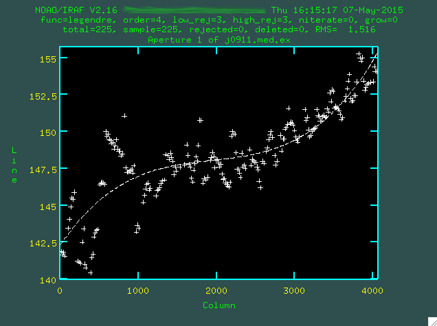
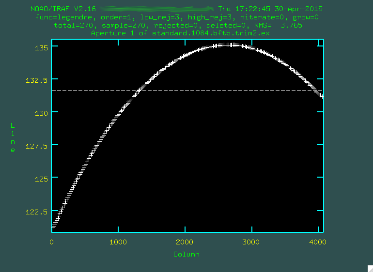
Fitcoords
transform in the next step. This
will be run using this line:
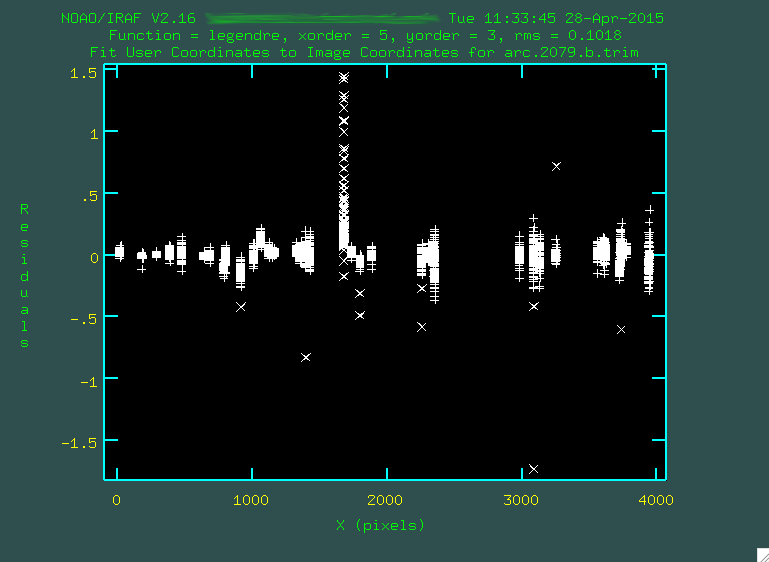
> fitcoords images=arc.2079.b.trim interactive=yes combine=no functio=legendre xorder=5 yorder=3
This step is run interactively, and you'll be presented with a window showing the fit.
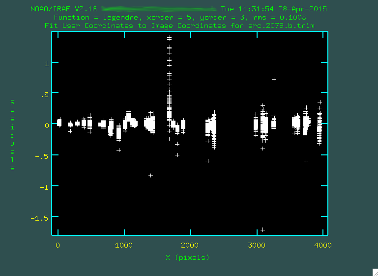
Each one of the bundles of points that you see corresponds
to a fitting of an arc emission line as a function of position up and down along
the spatial direction. The fit will try to go through all of
the points, and you can go through and remove outliers in a similar way to
how it was done in identify, by hovering over a point and pressing
d. However, instead of just deleting individual points, you are also given the option to delete
all of the points in the same x, y, or z coordinate. This is kind of a black box-ey
process. I've run this a bunch, and I mostly just make sure that the fit
does not seem to be overly dependent on some outlier points, and then I call it
a day. You can also change the order of the fit using :xor X or :yor X, where
X is the new fit.
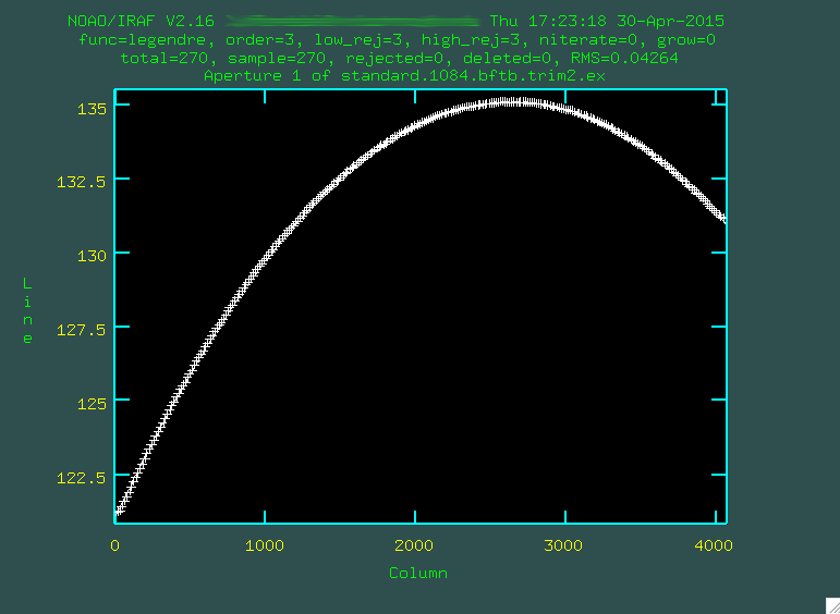
For the fit above, I definitely didn't like that one column of outlying points,
so I deleted it by hovering over one of the points in the column and typing d
and then z. I also deleted some of the individual outlier points by
hovering over them and typing d and then p.
Remember after each point deletion, to press "f" to re-fit the function to the remaining points. When you're happy, press "q", and you'll get some screen output:
  NOAO/IRAF V2.16 yourusername@yourcomputer Tue 11:31:54 28-Apr-2015
    Longslit coordinate fit name is arc.2079.b.trim.
    Longslit database is database.
    Features from images:
      arc.2079.b.trim
    Map User coordinates for axis 1 using image features:
    Number of feature coordnates = 4279
    Mapping function = legendre
     X order = 5
      Y order = 3
    Fitted coordinates at the corners of the images:
      (1, 1) = 6885.995  (4064, 1) = 3967.929
      (1, 1065) = 6885.536  (4064, 1065) = 3967.775
  Write coordinate map to the database (yes)?
You can use this to tell what the parameters of the fit are. Say
yes when the program asks to write the coordinate map to the database. As with
identify, this will produce a file in the database folder, and
in our case for the example, the file is called fcarc.2079.b.trim.
Initial Science Image Reduction
The first step we'll take with our science images, is, of course, to bias subtract them. I have three 1800s science exposures:
  % perl bias_4k.pl j0911.1076.fits
  % perl bias_4k.pl j0911.1077.fits
  % perl bias_4k.pl j0911.1078.fits
Take a look at the results (here's an example: j0911.1076.b.fits). Now that we've bias subtracted the images, we can remove whatever tiny amount of dark current exists in the images by subtracting the bias-subtracted combined dark image from above. For the remainder of this explanation, I will not be doing this, but if you did, you'd run the process like this:
  > imarith j0911.1076.b.fits - dark_combine.fits j0911.1076.bd.fits
  > imarith j0911.1077.b.fits - dark_combine.fits j0911.1077.bd.fits
  > imarith j0911.1078.b.fits - dark_combine.fits j0911.1078.bd.fits
Notice where I am keeping the file dark_combine.fits, and what I am calling the dark subtracted image (".bd."), to let me know that I have run dark reduction. This naming convention also allows me to quickly list the images when I want to move them somewhere. HOWEVER, because I won't be running dark subtraction from here on out, I won't have that extra "d" in the file name.
Before I flatten the images, I have to trim them, using the same region that I used when I made the flat:
  > imcopy j0911.1076.b.fits[1:4064,1500:2564] j0911.1076.b.trim.fits
  > imcopy j0911.1077.b.fits[1:4064,1500:2564] j0911.1077.b.trim.fits
  > imcopy j0911.1078.b.fits[1:4064,1500:2564] j0911.1078.b.trim.fits
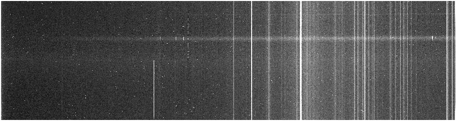
Again, take a look (j0911.1076.b.trim.fits). Notice that you can see the actual trace of the spectrum going from left to right, with some little emission lines. Next, I divide by the flat I chose, flatnorm.1.fits:
  > imarith j0911.1076.b.trim.fits / flatnorm.1.fits j0911.1076.bf.trim.fits
  > imarith j0911.1077.b.trim.fits / flatnorm.1.fits j0911.1077.bf.trim.fits
  > imarith j0911.1078.b.trim.fits / flatnorm.1.fits j0911.1078.bf.trim.fits
Before we move on, notice that I divided by flatnorm.1.fits as if it were in the same folder as the images we're working with. To make things more clean, you can put the flats in their own folder, and the point to where they are. For instance, if they're in a folder called "flats/" then I'd use:
  > imarith j0911.1076.b.trim.fits / flats/flatnorm.1.fits j0911.1076.bf.trim.fits
  > imarith j0911.1077.b.trim.fits / flats/flatnorm.1.fits j0911.1077.bf.trim.fits
  > imarith j0911.1078.b.trim.fits / flats/flatnorm.1.fits j0911.1078.bf.trim.fits
Instead. However you do it (and again, I recommend keeping things separate since
it makes looking at the data later on a lot more straightforward), take a look
at the results (j0911.1076.bf.trim.fits).
It doesn't look too different from the original image, which is fine, the
flat fielding is a subtle, but important effect.
You can see some sky lines, but these will be removed when we run the
background task later.
Cosmic Ray Zapping
While this step is not technically necessary if you have three or more
images, I like to create "bad pixel masks" for each of the images that point out
where the cosmic rays and bad pixels effect the final data. Long exposure data
is prone to having a great deal of cosmic rays, and we can use the IRAF task
xzap to find and remove them.
xzap is native to IRAF, so if you don't have
xzap installed, you can download a
zip file containing the script here. Open that up and put the contents into
a folder with your other IRAF user scripts (if you don't have an IRAF scripts
folder, you should). Then, in your loginuser.cl file, you need to call these:
  task xzap  = "scripts$xzap.cl"
  task fileroot = "scripts$fileroot.cl"
  task iterstat = "scripts$iterstat.cl"
  task makemask = "scripts$makemask.cl"
  task minv = "scripts$minv.cl"
(Notice that I have
scripts there in the path to the scripts.
The first line in my scripts file is set scripts = home$scripts/,
because my scripts folder is located within the home IRAF folder, and that's
where all of these .cl files live. Also, at the bottom of your loginuser.cl
file, you should put the word keep. So, a full loginuser.cl file
that's built just to run xzap would look like this:
  set scripts = home$scripts/

  task xzap  = "scripts$xzap.cl"
  task fileroot = "scripts$fileroot.cl"
  task iterstat = "scripts$iterstat.cl"
  task makemask = "scripts$makemask.cl"
  task minv = "scripts$minv.cl"

  keep
Now you should be able to run
xzap.
This task looks
at a background level across the image, and finds those pixels that have
sharp, bright count levels and then marks them, grows a buffer region around them,
and then fills these regions in using median filtering. The program produces two
files, one being the image with cosmic rays reduced, and the other being a
cosmic ray mask (providing you haven't told the program to delete this file),
which you will use when running imcombine.
Here are the parameters that I use when looking at OSMOS data:
  PACKAGE = noao
  TASK = xzap

  inlist  =   j0911.1078.bf.trim  Image(s) for cosmic ray cleaning
  outlist =  j0911.1078.bfz.trim  Output image(s)
  (zboxsz =                    6) Box size for zapping
  (nsigma =                   9.) Number of sky sigma for zapping threshold
  (nnegsig=                   0.) Number of sky sigma for negative zapping
  (nrings =                    2) Number of pixels to flag as buffer around CRs
  (nobjsig=                   2.) Number of sky sigma for object identification
  (skyfilt=                   15)   Median filter size for local sky evaluation
  (skysubs=                    1)   Block averaging factor before median filtering
  (ngrowob=                    0)   Number of pixels to flag as buffer around objects
  (statsec=    [XXX:XXX,YYY:YYY]) Image section to use for computing sky sigma
  (deletem=                   no) Delete CR mask after execution?
  (cleanpl=                  yes) Delete other working .pl masks after execution?
  (cleanim=                  yes) Delete working .imh images after execution?
  (verbose=                  yes) Verbose output?
  (checkli=                  yes) Check min and max pix values before filtering?
  (zmin   =              -32768.) Minimum data value for fmedian
  (zmax   =               32767.) Minimum data value for fmedian
  (inimgli=                     )
  (outimgl=                     )
  (statlis=                     )
  (mode   =                   ql)
Here, the important values to fiddle with are the first five. You're going to want to examine the output image against the input image, as well as the mask, which will be given the name "crmask_j0911.1078.bf.trim.pl" in our example above.
You're also going to want to change the "statsec" section. The format of
the statsec is [XXX:XXX,YYY:YYY], where XXX:XXX is the xmin and xmax "image" pixel
values, and YYY:YYY is the ymin and ymax "image" pixels values of a region
on the image without any signal from the trace, but near it. For the object
we're examining in the example data, I used [2000:2200,400:600]. You can also
specify the statsec when you call xzap, and I'll demonstrate that
below.
If you run the cosmic ray zapping before transforming your data, you will have to include your mask to be transformed along with the data. If you run cosmic ray zapping after transforming the data, you've moved around some of the cosmic ray flux, which is non-ideal, so always run it beforehand.
Here is how I call xzap:
  > xzap j0911.1076.bf.trim j0911.1076.bfz.trim statsec=[2000:2200,400:600]
  > xzap j0911.1077.bf.trim j0911.1077.bfz.trim statsec=[2000:2200,400:600]
  > xzap j0911.1078.bf.trim j0911.1078.bfz.trim statsec=[2000:2200,400:600]
This will take a bit, and produce some output to the screen, like this for 1076:
  Working on j0911.1076.bf.trim ---ZAP!--> j0911.1076.bfz.trim
       Computing statistics.
  j0911.1076.bf.trim[2000:2200,400:600]: mean=4.243423  rms=9.20291  npix=40401  median=4.09466  mode=3.928187
  j0911.1076.bf.trim[2000:2200,400:600]: mean=4.157449  rms=2.251932  npix=40392  median=4.088549  mode=4.02332
  j0911.1076.bf.trim[2000:2200,400:600]: mean=4.153667  rms=2.227629  npix=40383  median=4.019503  mode=3.958442
  j0911.1076.bf.trim[2000:2200,400:600]: mean=4.15339  rms=2.226962  npix=40382  median=4.044592  mode=3.969862
       Median filtering.
       Data minimum = -733.78778076172  maximum = 58121.3515625
       Truncating data range -733.78778076172  to 32767.
       Masking potential CR events.
       Creating object mask.
       Thresholding image at level 4.43246914
       Growing mask rings around CR hits.
       Replacing CR hits with local median.
  add j0911.1076.bf.trim,CRMASK = crmask_j0911.1076.bf.trim.pl
  add j0911.1076.bfz.trim,CRMASK = crmask_j0911.1076.bf.trim.pl
       Done.
This is normal, and you can suppress this output to the screen by setting
verbose = no in the parameters or when you call xzap.
The results for 1076 are below:
 Before cosmic ray zapping (j0911.1076.bf.trim.fits)
 After cosmic ray zapping (j0911.1076.bfz.trim.fits)
 Cosmic ray mask (crmask_j0911.1076.bf.trim.pl)
It's important that the cosmic ray zapping doesn't mask off emission
features, or parts of a bright trace (if your central trace is, indeed super
bright). If that happens, you need to go back and change the sigma values in
the xzap procedure and re-run everything. Eventually, you'll
get something that looks good. Now, what's interesting is that even though
we produced *.bfz.trim.fits files, we won't be using them
if we have three or more images, because we can use median combining at the
end. If you just have two images in a set, you'll have to use these cosmic
ray zapped images going on, because you can't take a median with only
two images.
Transform
Ok! Now, we'll transform our science image using the output database from
fitcoords, using the IRAF task transform, found in noao.twodspec.longslit:
  > transform input=j0911.1076.bf.trim.fits output=j0911.1076.bft.trim.fits minput=crmask_j0911.1076.bf.trim.pl moutput=crmask_j0911.1076.bft.trim.pl fitnames=arc.2079.b.trim interptype=linear flux=yes blank=INDEF x1=INDEF x2=INDEF dx=INDEF y1=INDEF y2=INDEF dy=INDEF
  > transform input=j0911.1077.bf.trim.fits output=j0911.1077.bft.trim.fits minput=crmask_j0911.1077.bf.trim.pl moutput=crmask_j0911.1077.bft.trim.pl fitnames=arc.2079.b.trim interptype=linear flux=yes blank=INDEF x1=INDEF x2=INDEF dx=INDEF y1=INDEF y2=INDEF dy=INDEF
  > transform input=j0911.1078.bf.trim.fits output=j0911.1078.bft.trim.fits minput=crmask_j0911.1078.bf.trim.pl moutput=crmask_j0911.1078.bft.trim.pl fitnames=arc.2079.b.trim interptype=linear flux=yes blank=INDEF x1=INDEF x2=INDEF dx=INDEF y1=INDEF y2=INDEF dy=INDEF
Notice that we're specifying our arc lamp in the fitnames parameter. This
requires us to have both the arc image and the database folder in the directory
where we're working. If you've been following along, these files are already
in your working directory, so don't worry. Sometimes, though, you might want
to use the transform for one set of files on another set, and you're going to
have to copy the whole database directory and the arc file. The transform
program takes a bit to run depending on the size of the image, and near the end it
will ask for the dispersion axis, which in this case is (1), along the lines.
When it runs, take a look at the result. The sky lines should be straight up and
down, or else something has gone wrong.
If you've run cosmic ray zapping, notice that the masks are also transformed
with the minput and moutput parameters.
If you were to open the resulting *bft.trim.fits file within
ds9 itself, you would be able to see that value for WCS appears when you mouse
over the image. (Important Note: if you open the file from IRAF, then you
won't see the wavelengths, because IRAF has a hard time with this, in both
images and spectra) This is the wavelength of that point in the image. It should not
change as you move up and down in the image at a single x value, since that
was how the transformation was defined. If you mouse over the various emission
lines, you can get an idea of what the observed wavelength is for them! Look
for the [OIII] 5007 line, which for this object (z = 0.027, remember), should
be observed at 5142 Angstroms.
Trimming (Again) and Background Subtraction
Now, we'll just go and run the actual background subtraction on the images. The "background" is all of the underlying light that has made it through the slit from sources that are not the source. In general, this tends to be the brightness of the sky itself, which glows across the whole wavelength range, and also in very specific emission lines that you can see as the big vertical white bands that are dominant in the red part of the spectrum.
We're going to use the IRAF taskbackground to do this, which will
fit the regions on either side of the central trace, and then apply this model
to the whole two-dimensional spectrum, subtracting both continuum and sky lines,
leaving just the spectrum of the object we care about.
However, beforehand, let's just really trim the image so it's only the spectrum.
We do this because background can take a long time to run, and we only really
care about a region that's near the spectrum, where we can see signal. We should
make sure, however, that we leave a good amount of space above and below the line:
  > imcopy j0911.1076.bft.trim.fits[1:4064,580:880] j0911.1076.bft.trim2.fits
  > imcopy j0911.1077.bft.trim.fits[1:4064,580:880] j0911.1077.bft.trim2.fits
  > imcopy j0911.1078.bft.trim.fits[1:4064,580:880] j0911.1078.bft.trim2.fits

  > imcopy crmask_j0911.1076.bft.trim.pl[1:4064,580:880] crmask_j0911.1076.bft.trim2.pl
  > imcopy crmask_j0911.1077.bft.trim.pl[1:4064,580:880] crmask_j0911.1077.bft.trim2.pl
  > imcopy crmask_j0911.1078.bft.trim.pl[1:4064,580:880] crmask_j0911.1078.bft.trim2.pl
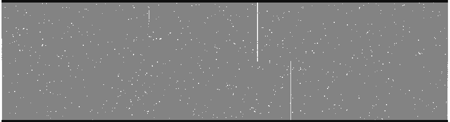
Notice that I've also trimmed the transformed masks as well! Here's an example of both:


And now, with those files created, let's run background:
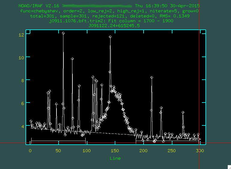
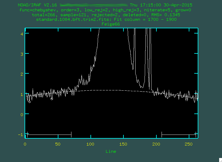
  > background input=j0911.1076.bft.trim2 output=j0911.1076.bftb.trim2 axis=2 interactive=yes naverage=1 function=chebyshev order=2 low_rej=2 high_rej=1.5 niterate=5 grow=0
  > background input=j0911.1077.bft.trim2 output=j0911.1077.bftb.trim2 axis=2 interactive=yes naverage=1 function=chebyshev order=2 low_rej=2 high_rej=1.5 niterate=5 grow=0
  > background input=j0911.1078.bft.trim2 output=j0911.1078.bftb.trim2 axis=2 interactive=yes naverage=1 function=chebyshev order=2 low_rej=2 high_rej=1.5 niterate=5 grow=0
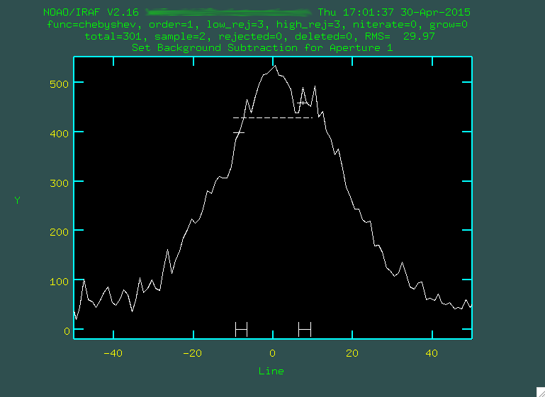
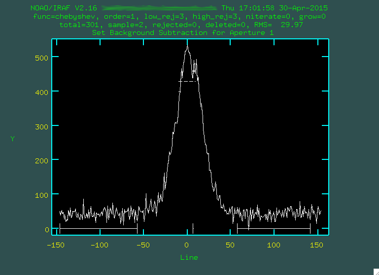
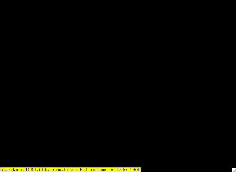
We want to do this interactively, and you'll first be presented with a black screen:
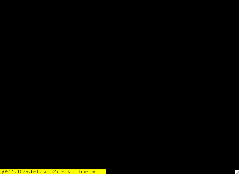
You want to type the X values (or Y values, depending on the
dispersion axis) that straddles some bright portion of the spectrum. In
our case, let's go with a region just to the red of [OIII] 5007,
between 1700 and 1900, so just type 1700 1900, and then press enter.
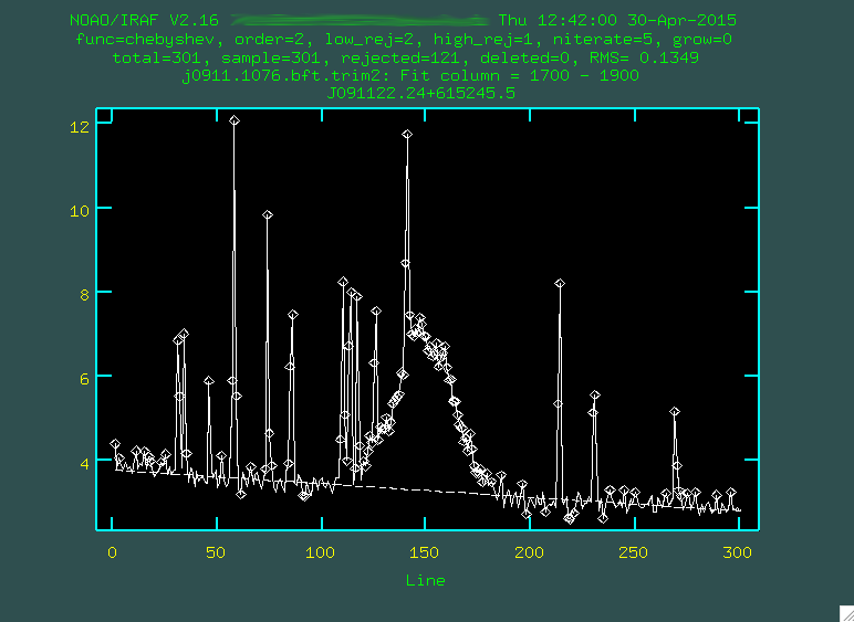
s at the leftmost
part of a region that contains the background, and then s at a
point to the right of where the background is. So, for instance, I clicked
s here:
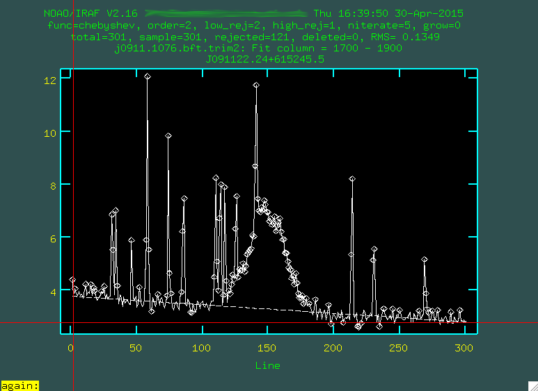
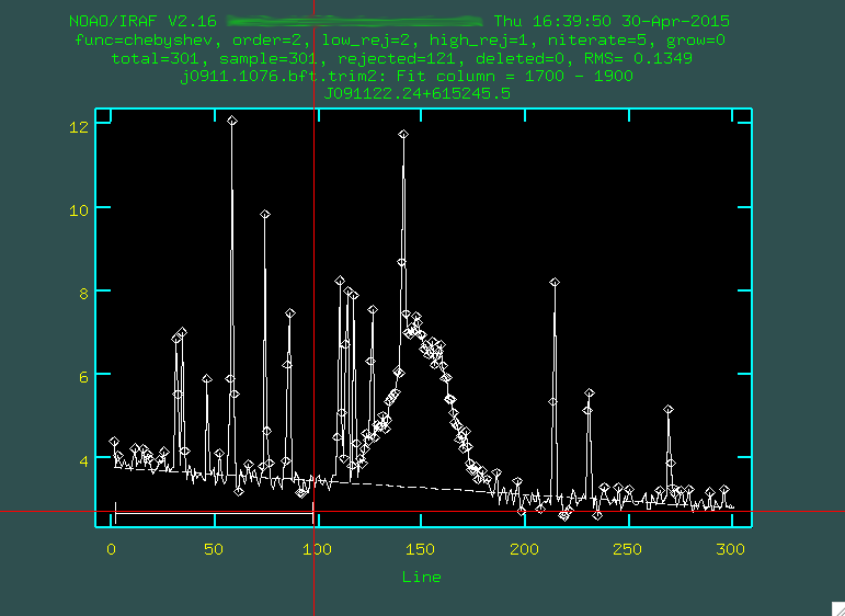
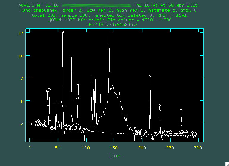
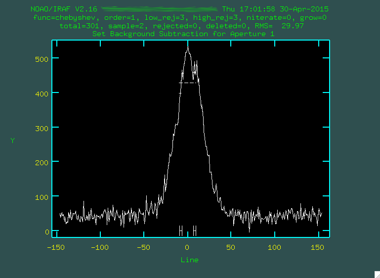
:or 3 (or 4, or 5 or
whatever you think fits best, I'm going to go with 3), then you re-fit by typing f:
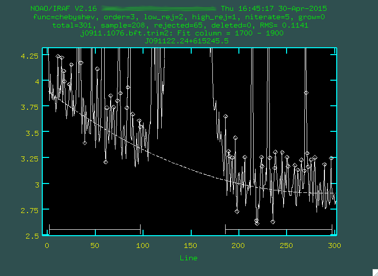
identify, by typing w then e on
the bottom left corner of the zoomed in region I want, and then e on the top right corner of the zoomed
in region I want.
If it does to your liking, press q and then press the enter key.
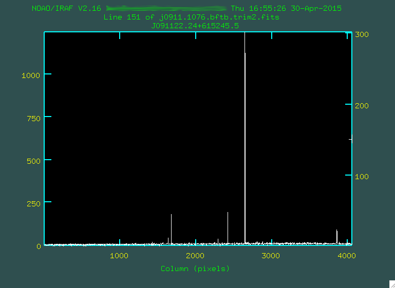
The background subtraction will take a little while, but when it's done, take a look at the result. The sky lines should be gone, and the background level should be noisy, but zero-ish. You'll still see the cosmic rays, which we'll deal with in the next step:

You can use implot
to look and see that the background is actually zero, by typing:
> implot j0911.1076.bftb.trim2.fits
You can just plot a column of interest by typing something like
:c 1500 2000, which will plot columns 1500 to 2000
collapsed, and should very similar to what you saw when you were background
subtracting, but the background levels have been subtracted out.
Now, once you've done this for all of the images, let's imcombine the data.
Imcombine Science Images
Here, we are going to use imcombine, along with our bad pixel masks, to
create a combined science image, as well as an error image. Before we combine
the images, we have to make sure that the image header has the trimmed bad
pixel mask. When imcombine takes the three science exposure and
combines them, it will use the bad pixel masks given using the BPM
header keyword. So, first, let's take a look at the header, using imhead:
> imhead j0911.1076.bftb.trim2.fits l+
Here, l+ tells IRAF that you want the whole header.
Scroll down (in IRAF, scrolling is accomplished through a "middle click", which
you can do on a Mac by holding down option while you click on the scroll bar.) and
look for the header keyword BPM:
BPM = 'crmask_j0911.1076.bft.trim.pl'
Now, we want this to actually have crmask_j0911.1076.bft.trim2.pl,
instead, so we can use the IRAF task ccdhedit, found in noao.imred.ccdred:
> ccdhedit j0911.1076.bftb.trim2.fits BPM "crmask_j0911.1076.bft.trim2.pl"
Now, if you check the image header (same as above, use imhead and
l+, and you'll hopefully see that the BPM header
now reads crmask_j0911.1076.bft.trim2.pl. The second way that you
can edit the image header is using the IRAF task eheader, found in
stsdas.toolbox.headers:
> eheader j0911.1076.bftb.trim2.fits
This is going to open up the whole image header for you to edit. By default, the
editor that IRAF uses is vim, which is a pretty
crazy text editor. If you want to edit anything, move the cursor down to where
you want to make the edit using the up/down/left/right arrows on the keyboard,
then press i to go into "insert mode," and now you can add in
the text you want (like the 2 in our example above), and then you press esc
to escape out of insert mode, and then finally :wq to save and quit
the image header editing. It's a bit of a process.
So, now that the image headers are fixed, we can move on to imcombine.
First, take a look at the individual exposures. Specifically, you want to make
sure that the object didn't move up or down along the slit between the three exposures.
If that's the case, you can't just stack the images, but instead you have to
include an alignment file that tells imcombine how to offset each
image. The MDM 2.4m has a pretty good tracking system, so this is often an
entirely unnecessary procedure, but here's a way to generate an alignment file
in case you somehow need to.
If you have a bright emission line in each image, you could load each
*.bftb* image into ds9:
> displ j0911.1076.bftb.trim2.fits 1 fill+
At this point, you can use the IRAF task imexamine to find the centroid
for that bright emission line:
> imexamine j0911.1076.bftb.trim2.fits
This will change your mouse cursor to a little annulus when you hover over ds9.
At this point, put the mouse over the emission feature on the image and
type a. You'll see output like this (which is for the [OIII] feature
from :
 Here's the output for doing this for
 j0911.1076.bftb.trim2.fits,
j0911.1077.bftb.trim2.fits, and j0911.1078.bftb.trim2.fits:
  #   COL    LINE       COORDINATES     R    MAG    FLUX     SKY    PEAK    E   PA      ENCLOSED GAUSSIAN DIRECT
  1633.68  157.59 5140.438 736.5936  13.69  10.51   6770.   2.814   196.4 0.69  -88          5.85     4.59   4.56
  1633.34  158.76 5140.19  737.7632  13.58   9.82  12821.   4.664   400.9 0.71  -88          5.55     4.47   4.53
  1633.12  159.75 5140.032 738.748   14.50  10.04  10454.   4.026   262.8 0.67  -88          6.56     4.83   4.84
The most important thing are the first two columns from the output, which are the X
and Y positions of the centroid for the feature. In this case, while the feature
doesn't shift too much in the X direction, it does move upward by a couple of
pixels. Again, I normally don't worry about this too much, especially since
the imexamine procedure was designed to work on stars, not
emission lines.
There is another potential way to align everything. You can use implot,
as described above, to look at the continuum, and match based on that:
> implot j0911.1076.bftb.trim2.fits
And then, look at some range in columns that have strong continuum by typing
:c 1494 1554. This will collapse the 2D spectrum between these
pixel values in the dispersion direction and show you the summed trace
between the two.
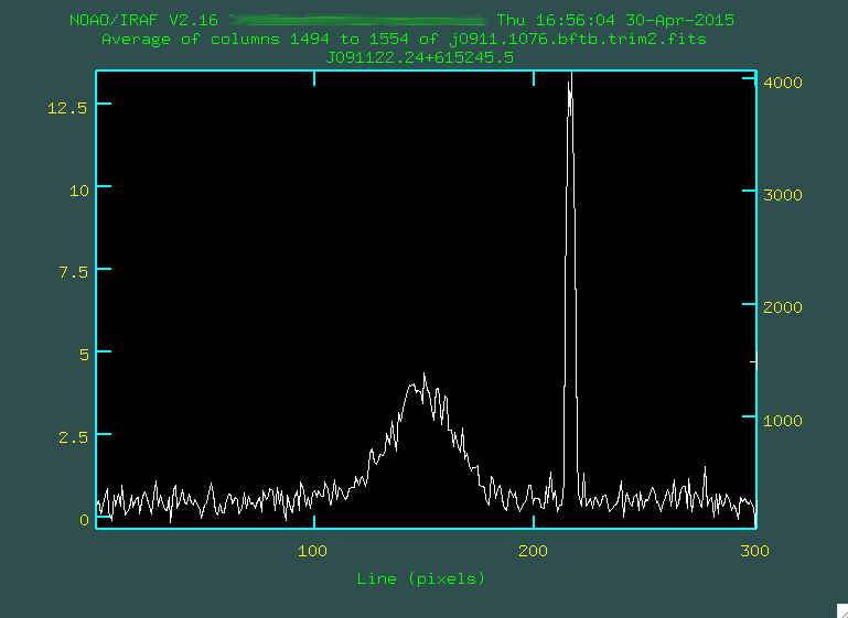 Here, the x axis represents the up/down (spatial) pixel value in the image, and
the central hump is the trace. The big spike there on the right is a bad pixel
or two. You can go and move your mouse cursor over a spot that looks to be
the peak, and press the space bar:
Here, the x axis represents the up/down (spatial) pixel value in the image, and
the central hump is the trace. The big spike there on the right is a bad pixel
or two. You can go and move your mouse cursor over a spot that looks to be
the peak, and press the space bar:
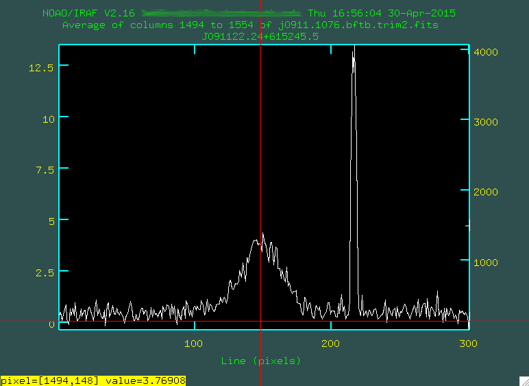 Now you'll see the position, and the 2D spectra value for where you put the cursor,
which in this case is [1494, 148], with a value of 3.769. This means that the
center of the trace is about 148 for this image. If I do this for the other
two images, I get 149 and 150. This is real small, and agrees with what we see
above, about a one pixel shift per image.
Now you'll see the position, and the 2D spectra value for where you put the cursor,
which in this case is [1494, 148], with a value of 3.769. This means that the
center of the trace is about 148 for this image. If I do this for the other
two images, I get 149 and 150. This is real small, and agrees with what we see
above, about a one pixel shift per image.
If we wanted to align everything when running imcombine, our
offsets file would look, then, like this:
  0 0
  0 -1
  0 -2
Here, we want to shift everything to the first file (1076), and the other two are one and two pixels off from that. You would then save this to a file (I tend to call it "offsets.list").
Now, let's take the science images and put them into a file:
> ls *bftb* > j0911.list
Now, when we run imcombine, we're going to want to scale the images
before we median combine them. Otherwise, if there was an image that was systematically
lower than the other two, then a median combine wouldn't provide an accurate
final image. Ideally, the images were all taken with the same exposure time, so
the scaling should be minimal. We want to calculate the scaling using a region
of the image with just the background, similar to how we ran xzap. I
have chosen the region between pixels 1394 and 1513 in the x direction, and
200 to 260 in the y-direction. We'll set this as our statsec.
And finally, let's run imcombine. If we want to run it without
an offsets file, we'd run:
> imcombine @j0911.list j0911.med.fits sigma=j0911.med.sig.fits combine=median scale=mean statsec=[1394:1513,200:260] masktype=goodvalue
And if we wanted to run this without an offsets file, we'd run:
> imcombine @j0911.list j0911.med.fits sigma=j0911.med.sig.fits offsets=offsets.list combine=median scale=mean statsec=[1394:1513,200:260] masktype=goodvalue
Notice that we are using a median combine. If we had only two images, we'd want
to run combine=average instead. Also notice that we've created
a "sigma" image, which is the basis for our output error spectrum. We set
masktype=goodvalue which means that it
uses the bad pixel masks we created earlier to mask out the bad pixels for each
image.
When we run the line, the screen will output some information:
  Apr 30 13:10: IMCOMBINE
    combine = median, scale = mean, zero = none, weight = none
    blank = 0.
    masktype = goodval, maskval = 0
                  Images     Mean  Scale Maskfile
    j0911.1076.bftb.trim2.fits 0.45086  1.000 crmask_j0911.1076.bft.trim2.pl
    j0911.1077.bftb.trim2.fits 0.36008  1.252 crmask_j0911.1077.bft.trim2.pl
    j0911.1078.bftb.trim2.fits 0.42913  1.051 crmask_j0911.1078.bft.trim2.pl

    Output image = j0911.med.fits, ncombine = 3
    Sigma image = j0911.med.sig.fits
This is mostly important for showing how it scaled the images. Either way,
let's take a look at the final image:


This looks pretty good! We have a strong continuum, with some prominent emission lines. The ringing comes from both the transformation, and the fact that the sigma image has had a standard deviation used in its estimation.
Make The Variance Image
This is a straightforward step. We're going to take the recently created sigma image, and turn it into a variance image. We'll use this to extract error variance spectra, which we can turn into sigma spectra:
  > imcalc j0911.med.sig.fits j0911.med.sig.sqr.fits "im1**2"
  > imcalc j0911.med.sig.sqr.fits j0911.med.var.fits "im1/3"
  > imdel j0911.med.sig.sqr.fits
So, here, we are first taking the square of the sigma image, and then dividing by the number of images that went into making it, which creates the variance image. Finally, we delete the squared image. In a future step, when we extract a spectrum from the variance image, we're going to want to take the square root of it to get the sigma spectrum, which is our true uncertainty on the spectral values.
Extinction Correction
So, before we extract, we can run extinction correction based on the
airmass. We'll use the extinction program, which is part of the
noao.twodspec.longslit package:
  PACKAGE = longslit
     TASK = extinction

  input   =   j0911.med.var.fits  Images to be extinction corrected
  output  = j0911.med.var.ex.fits  Extinction corrected images
  (extinct= onedstds$kpnoextinct.dat) Extinction file
  (mode   =                   ql)
So, you can see here that we've set extinct=onedstds$kpnoextinct.
which is the kitt peak standard extinction file. You run the program in this way:
  > extinction j0911.med.fits j0911.med.ex.fits
  Extinction correction: j0911.med.fits -> j0911.med.ex.fits.
This will run using the Zenith Distance (given as ZD in the header), in a way described here. Make sure to run this same process on the variance image, as well:
  > extinction j0911.med.var.fits j0911.med.var.ex.fits
  Extinction correction: j0911.med.var.fits -> j0911.med.var.ex.fits.
Aperture Extraction
Now that we have our stacked 2D spectrum, we want to extract a 1D spectrum.
For aperture extraction, we'll be using the IRAF program
apall, which is part of the noao.twodspec.apextract
package. I have put a .cl script here,
which we'll use to extract our 1D spectrum.
apall.
Apall will look for a peak in some column range that we give it (the first part
will look a lot like our implot runs above. Then, armed with this
position of the central trace in the spatial (up and down) direction, it will
trace the whole spectrum in the wavelength direction.
So, open up apall.sci.cl in your favorite editor. First, we're
going to want to change apall.input to the name of the reduced
fits file we just created, and change the output to be whatever we want.
  apall.input="j0911.med.ex.fits"
  apall.nfind=1
  apall.output="j0911.med.ex.ms"
  apall.apertures=""
  apall.format="multispec"
  apall.references=""
  apall.profiles=""
Next we'll want to make sure that a series of flags are set correctly for
what we want to do on the first pass. We want to do this interactively, and we
want the program to find the central aperture. We don't need to recenter, or
resize, but we'd like to edit the apertures (so we can look at them). We want to
trace the aperture in the velocity direction, and fit to that trace, and finally,
we want to extract the aperture.
  apall.interactive=yes
  apall.find=yes
  apall.recenter=no
  apall.resize=no
  apall.edit=yes
  apall.trace=yes
  apall.fittrace=yes
  apall.extract=yes
  apall.extras=no
  apall.review=no
Now, these next lines are important. apall.line
should be set to the central row/column pixel value of the range you care about,
in pixel units. If you have a faint object, this might just be some bright
emission line. Here, since we have a pretty bright continuum, we can zero in on
that, and use a range near the [OIII] emission lines, since they're centrally
located on the image. The value for apall.nsum
is how many lines/columns you want to sum around that central pixel value.
Finally apall.lower and apall.upper
are the spatial size (in pixels) of the aperture on both sides of the center.
Generally you'll set these both to the same size.
So. If you want a twenty pixel wide aperture, and you want to look from 1450 -
1550 (which is between [OIII] 4959 and H-beta in our object), you'd set things
this way:
  apall.line=1500
  apall.nsum=100
  apall.lower=-10
  apall.upper=10
Leave the rest as it is, as it's stuff relating to the trace, and weights,
but change the final line, so that apall is actually called:
apall j0911.med.ex.fits
So, now, we can run the script:
> cl < apall.sci.cl
This should run the script. If this doesn't work for some reason, the
script can be opened, and the IRAF parameter file for apall
can be set by hand based on what's in the script. Then you can run apall
in any way that works.
The program is going to ask some questions:
  Find apertures for j0911.med.ex?  (yes):
  Number of apertures to be found automatically (1):
  Edit apertures for j0911.med.ex?  (yes):
You set all of this in the script, so you can probably press "enter" to go
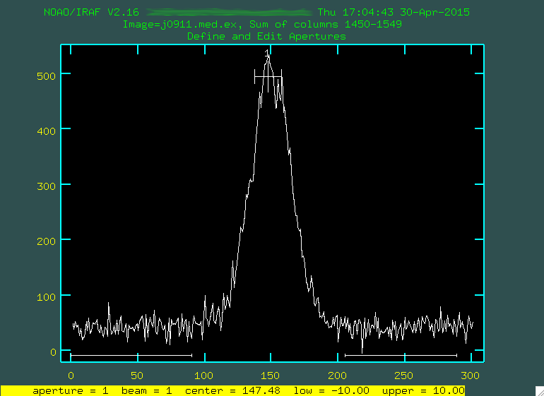
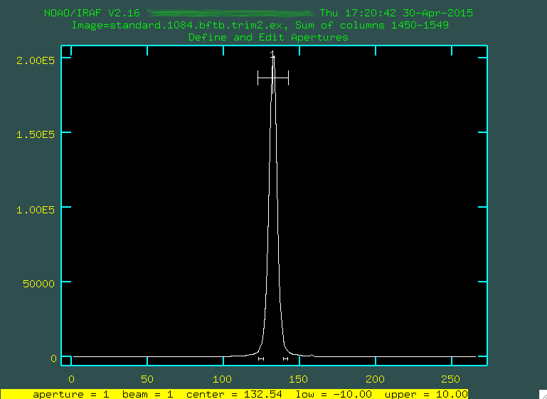
through this all. You'll eventually get to the a screen showing the aperture:
 Now, what we're seeing is the program's attempt to find the trace in our
region we've specified with
Now, what we're seeing is the program's attempt to find the trace in our
region we've specified with apall.line, which, in our case, is this
bright peak at the very center. You can see that it's essentially found this peak,
since there's a little region marked off at the top labeled "1". You can see the
width we've given it (+/- 10 pixels) as the little whiskers to the right and
left on the symbol. If you want to widen it at all, you can move the cursor to the position along the curve
that represents the width you want and press y. If we weren't happy with this peak, we could hover over it
with the mouse and type d, which would delete this aperture, and
allow us to mark another one with n. In our case here, I'm fine
with this peak.
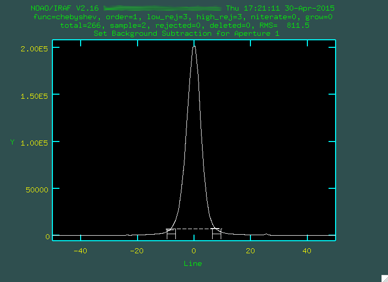
Now, notice the little bars right above the 150. These are the bars used to define
the background level for apall In our script, we set
apall.background="none", which meant that we didn't want to do
further background subtraction. If we had, instead, wanted to do more background
subtraction, we'd want to define the background outside of the trace. To do that,
we'd type b, and we'll be presented with this screen:
 From here, we're a little too zoomed in, so we can unzoom by again typing
 w n
and w m.
 Now, you can delete the original background regions by hovering over them
and typing
Now, you can delete the original background regions by hovering over them
and typing z. Then, you can mark new background regions exactly
like what was done using background earlier, by typing s
on either side of the regions you want to use. Here are my final regions for
defining the background:
 If I were happy with these regions, I would now want to type
 f:
 Then, if I was happy with the background I would type
 q. This should
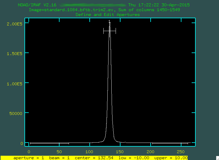
bring back the original screen:
 If you're happy with the central trace, and the background, again, type
 q.
The program will then ask if you want to trace the apertures, so type yes or
press "enter" if yes is already selected. You will be asked if you want to fit
the traced positions interactively, and we want to, so type yes, or
just press enter if yes is already given. You'll then be asked if you want to
fit a curve to aperture 1, and again, type yes or press enter if
yes is already selected.
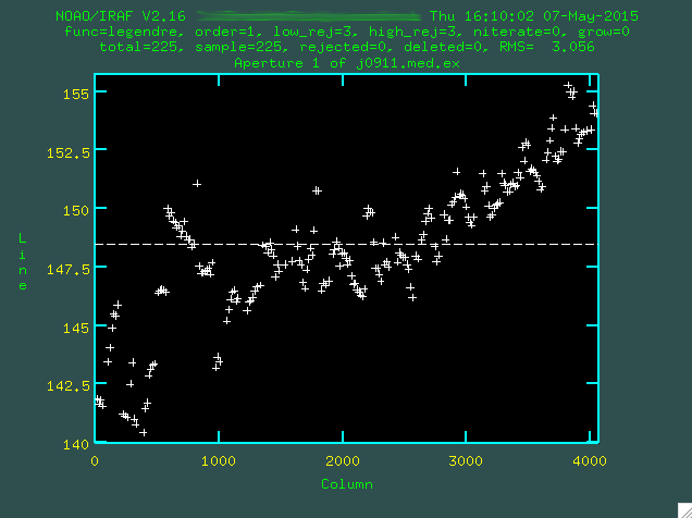
So, here, you are seeing the attempt by apall to find the trace
across the image. If you look at the scale on the left, you'll see that this is
a matter of pixels, and if you were go and look at j0911.med.ex.fits in ds9, you
would see that on the right side of the image, where the continuum is strongest,
it's actually at about a y position of 155, while on the left, where it's fainter,
it's actually a little lower. The dashed line is the initial fit to the trace,
which is not good. Let's go with a higher order polynomial. To do this,
type :or 4 (or whatever order you think is necessary), and then press enter,
and then re-fit with f.
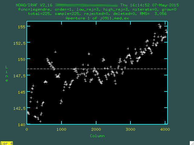
 Now, you can actually go and delete individual points with
 d if
you'd like, which is sometimes necessary near the edges of the images where
it's faint. In this case, you could go and delete a lot of the points on the
far left of the image, but for the purposes of this example, let's just go
with this fit.
As an aside, finding the trace, especially in faint targets, is kind of difficult
sometimes, and relies on a few parameters from the apall script. In
particular:
  apall.t_nsum=50
  apall.t_step=15
  apall.t_nlost=10
This is essentially saying, I want you to sum 50 lines in the dispersion direction,
in steps of 15 pixels, and most importantly, if you go 10 steps in the dispersion
direction and don't pick up a trace, quit. If this number is set too low, then
the trace will be lost and you won't be able to fit across the whole image. For
bright targets, you can set this lower, but generally it's good to keep it around
this value and double-check your final trace against the actual image to make
sure that it's not finding some spurious bright part of the image and saying
that this is the trace.
When you are happy with the fit, type q, and when asked if you
want to write the apertures to the database, type yes (or press
enter if yes is already selected), and then when asked if you want
to extract the aperture, type yes (or press enter if yes is already selected).
Now, take a look at that fit. You can use splot
to look at it:
> splot j0911.med.ex.ms.fits
Here we use .ms. to delineate one-dimensional spectra. Here is
our great spectrum:

This is a pretty handsome spectrum. You can see [OIII]4959,5007, H-beta, and the NII and H-alpha line complex! You can go and redo this to your hearts content if you're not happy with how that worked. The program has created a file in the folder "database", which in the case of the example is called "apj0911.med.ex". If you do want to redo the full extraction and tracing, delete this file first, so that the version we edit only has a record of one extraction, the last one that you did.
Now, we're going to want to go and extract an error spectrum. It's pretty straightforward. What you want to do first is copy over your apall.sci.cl script to another version that we'll call apall.sci.err.cl, for lack of a better name. We'll need to change a few things here:
  apall.input="j0911.med.var.ex"
  apall.nfind=1
  apall.output="j0911.med.var.ex.ms"
  apall.apertures=""
  apall.format="multispec"
  apall.references="j0911.med.ex"
  apall.profiles=""

  apall.interactive=no
  apall.find=no
  apall.recenter=no
  apall.resize=no
  apall.edit=no
  apall.trace=no
  apall.fittrace=no
  apall.extract=yes
  apall.extras=no
  apall.review=no
  ...
  apall j0911.med.var.ex.fits
Notice a few things. First, you are using a reference trace, which in this case is the trace you just extracted on the actual data. Also, you want to run this is noninteractive mode, you don't want to find, recenter, resize, edit, or fit to the trace. You do want to extract the spectrum, though! This will run the same exact aperture extraction as you just did, except on the variance image. So, run it:
> cl < apall.sci.err.cl
Once you extract a variance spectrum, you're going to want to turn this into a sigma spectrum to find the error at each wavelength:
> sarith j0911.med.var.ex.ms.fits sqrt "" j0911.med.sig.ex.ms.fits
Which takes the square root of the variance image and produces the sigma image, the error spectrum.
Flux Calibration
Our spectrum needs to be corrected for the response of the chip and the
units need to be converted to flux units. We can use our standard star observations
to do this. We'll quickly walk through the standard star reduction and extraction,
and then we'll use a suite of IRAF tasks, standard,
sensfunc, and calibrate,
to run the flux calibration.
We observed Feige 66, which is part of the IRAF/STSCI suite of standard stars
built in under onedstds$spec50cal/ see here
for a list of the standard stars from the STSCI package. We took one standard star
spectrum (standard.1084.fits), so the reduction is more straightforward than
it was for the science spectra. I tend to want to put the standard reduction
files into its own folder, but it's up to you.
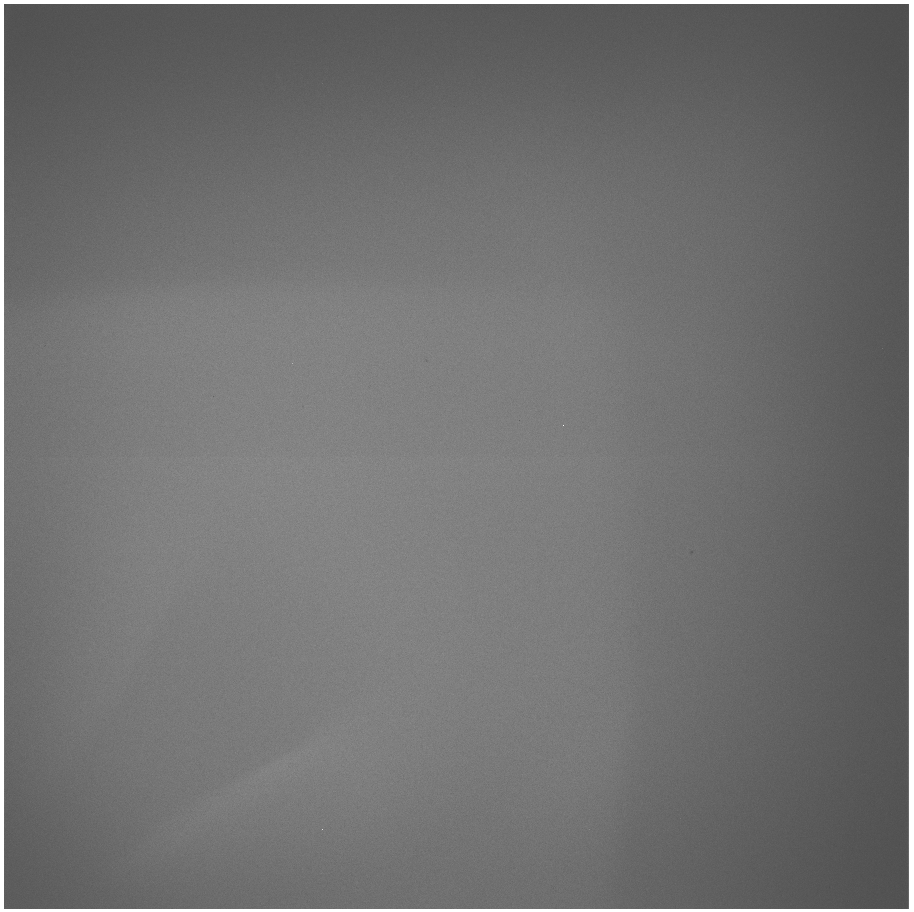
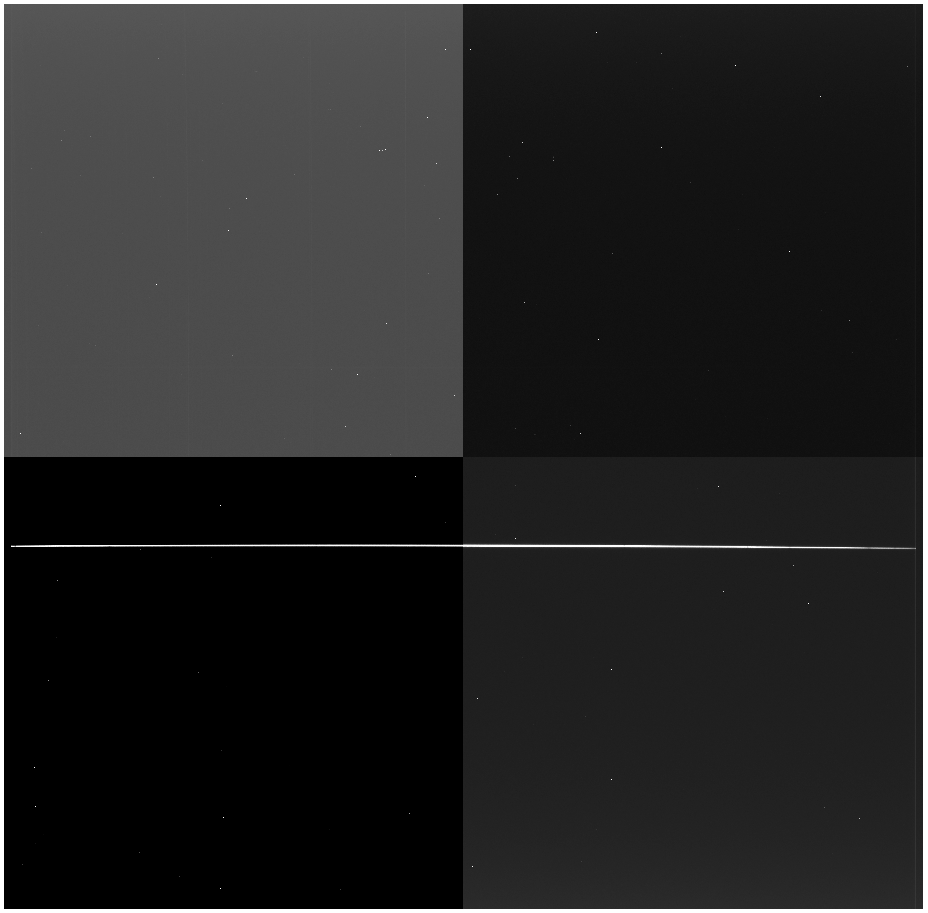 You can see the bright standard star trace running just below the chip gap.
Now, you'll start, of course, with bias subtraction:
You can see the bright standard star trace running just below the chip gap.
Now, you'll start, of course, with bias subtraction:
% perl bias_4k.pl standard.1084.fits
 Notice that there aren't very many cosmic rays, since this was only a
5 minute image. Next, we'll trim the image so we can flatten it:
Notice that there aren't very many cosmic rays, since this was only a
5 minute image. Next, we'll trim the image so we can flatten it:
> imcopy standard.1084.b.fits[1:4064,1500:2564] standard.1084.b.trim.fits
And here's the result:
 Here, the standard star is pretty low on the trimmed region, but since we trimmed
and calculated the wavelength solution using this same trimmed region, we have
to use it. In addition, this is the region we used to create the flat, which we
now want to use:
Here, the standard star is pretty low on the trimmed region, but since we trimmed
and calculated the wavelength solution using this same trimmed region, we have
to use it. In addition, this is the region we used to create the flat, which we
now want to use:
> imarith standard.1084.b.trim.fits / flatnorm.1.fits standard.1084.bf.trim.fits
And the result:

Since we have one image, we don't need to run cosmic ray zapping, especially
since the standard star is so bright. Instead, we'll transform the image. Before
we can do it, we have to bring over the database folder and the file arc.2079.b.trim.fits
from where we originally ran identify, reidentify,
and fitcoords. If they're in the folder with our new trimmed,
bias subtracted, flattened standard star spectrum, we can run transform:
> transform input=standard.1084.bf.trim.fits output=standard.1084.bft.trim.fits fitnames=arc.2079.b.trim interptype=linear flux=yes blank=INDEF x1=INDEF x2=INDEF dx=INDEF y1=INDEF y2=INDEF dy=INDEF
It should spit out some data to the screen, which, like all of the information printed out, should be copied to your log:
  NOAO/IRAF V2.16 yourusername@yourcomputer Thu 16:04:45 30-Apr-2015
    Transform standard.1084.bf.trim.fits to standard.1084.bft.trim.fits.
    Conserve flux per pixel.
    User coordinate transformations:
      arc.2079.b.trim
    Interpolation is linear.
    Using edge extension for out of bounds pixel values.
    Output coordinate parameters are:
      x1 =      3968., x2 =      6886., dx =     0.7182, nx = 4064, xlog = no
      y1 =         1., y2 =      1065., dy =         1., ny = 1065, ylog = no
Here is the resulting transformed standard star 2D spectrum:

Now, we'll want to trim again, before we remove the background:
> imcopy standard.1084.bft.trim.fits[1:4064,1:266] standard.1084.bft.trim2.fits
 Now, let's run the background subtraction:
> background input=standard.1084.bft.trim2.fits output=standard.1084.bftb.trim2.fits axis=2 interactive=yes naverage=1 function=chebyshev order=2 low_rej=2 high_rej=3 niterate=5 grow=0
You can use the same columns as before (1700 1900).
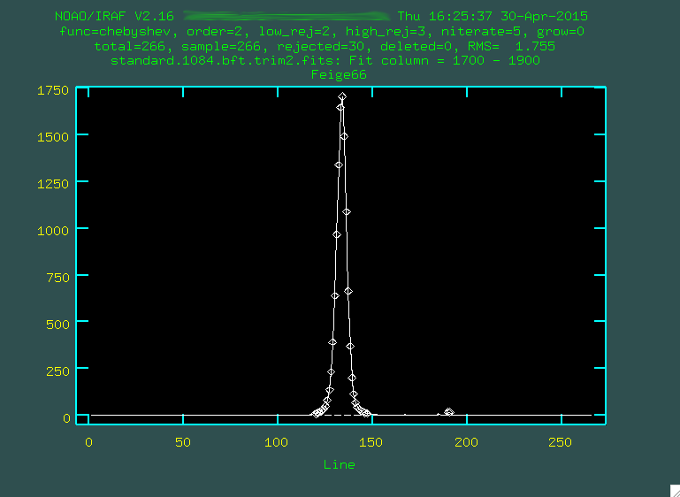 You can see the standard star trace there on the left, but you'll want to really
zoom in on the background:
You can see the standard star trace there on the left, but you'll want to really
zoom in on the background:
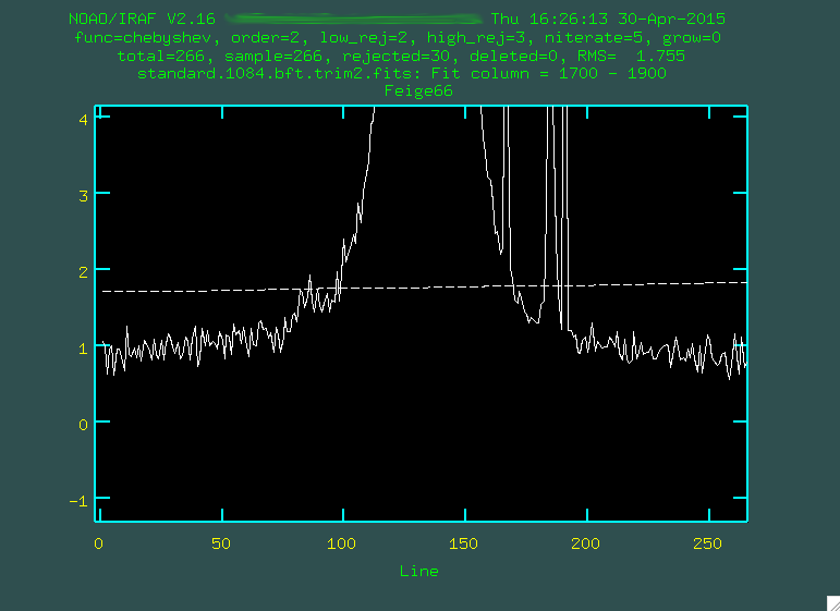 Now, like when we ran
 background on the science images, we'll want
to define the background correctly using s:
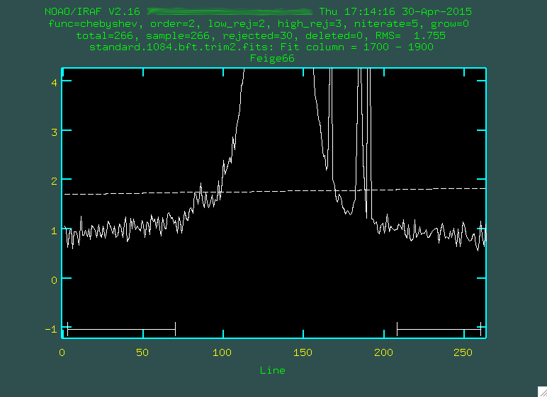
 In the second line, I also changed the fitting order to 3, using
 :or 3,
and then f. When I'm done, I type q, and then press enter,
and it'll remove the background:
 Next, we have to run the extinction correction:
  > extinction standard.1084.bftb.trim2.fits standard.1084.bftb.trim2.ex.fits
  Extinction correction: standard.1084.bftb.trim2.fits -> standard.1084.bftb.trim2.ex.fits.
Now, it's time to extract the standard star spectrum. You can use the same parameters as you would when you run the extraction of the actual spectrum. Just modify the apall.sci.cl script (I rename it apall.std.cl), and replace the input, output, and final lines of the script to use the file we just made:
  apall.input="standard.1084.bftb.trim2.ex.fits"
  apall.nfind=1
  apall.output="standard.1084.bftb.trim2.ex.ms.fits"
  apall.apertures=""
  apall.format="multispec"
  apall.references=""
  apall.profiles=""
  ...
  apall standard.1084.bftb.trim2.ex.fits
And then, we run it.
> cl < apall.std.cl
It's the same process as you ran with the science spectrum, but it could be that that trace is far stronger, so it should be easier.
 We start by typing
 b to define the background.
 After deleting the old background values with
 z, we zoom in using w and e:
 We define a new set of background regions using
 s, and then f to fit the background:
 When we're happy, we type
 q to go back to the original mode, and then
q again to move on to the part where it traces the region, making
sure that we allow it to trace by typing yes (or pressing enter) a few times.
 Now this is more like it. Look at that handsome, strong trace. We'll
want to use a higher order fit, I went with
Now this is more like it. Look at that handsome, strong trace. We'll
want to use a higher order fit, I went with :or 3:
 And it fit great! So, then I typed
 q, and pressed enter a few
times to allow apall to actually extract the spectrum.
Now you'll have a standard star spectrum (standard.1084.bftb.trim2.ex.ms.fits, if you're following along with my silly naming conventions):
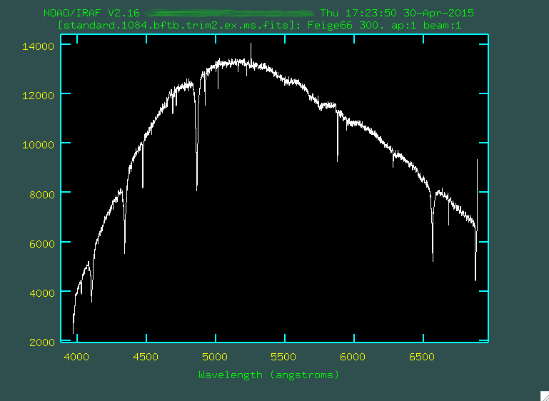 We can now, finally, begin the flux calibration. This standard star, as
mentioned above, is Feige 66 (which you can find from the log file, or
from the image header). Before we run
We can now, finally, begin the flux calibration. This standard star, as
mentioned above, is Feige 66 (which you can find from the log file, or
from the image header). Before we run standard, which is
found in noao.onedspec, we should edit one some specific
parameters, so let's open up the parameters for standard, with
epar standard.
  PACKAGE = longslit
     TASK = standard

  input   = standard.1084.bftb.trim2.ex.ms.fits  Input image file root name
  output  = standard.1084.bftb.trim2.ex.ms.out  Output flux file (used by SENSFUNC)
  (samesta=                  yes) Same star in all apertures?
  (beam_sw=                   no) Beam switch spectra?
  (apertur=                     ) Aperture selection list
  (bandwid=                INDEF) Bandpass widths
  (bandsep=                INDEF) Bandpass separation
  (fnuzero=  3.6800000000000E-20) Absolute flux zero point
  (extinct= onedstds$kpnoextinct.dat) Extinction file
  (caldir =  onedstds$spec50cal/) Directory containing calibration
                                  data
  (observa=       )_.observatory) Observatory for data
  (interac=                  yes) Graphic interaction to define new bandpasses
  (graphic=             stdgraph) Graphics output device
  (cursor =                     ) Graphics cursor input
  star_nam=              feige66  Star name in calibration list
  airmass =                       Airmass
  exptime =                       Exposure time (seconds)
  mag     =                       Magnitude of star
  magband =                       Magnitude type
  teff    =                       Effective temperature or spectral type
  answer  =                  yes  (no|yes|NO|YES|NO!|YES!)
  (mode   =                   ql)
On the page linked above (here, again,
but also you could just type help onedstds and see the same
information in IRAF) you can see that feige66 is under onedstds$spec50cal/,
and we would want to change the caldir to reflect the folder containing the standard
star used.
So, now, let's run standard:
  > standard
  Input image file root name (standard.1084.bftb.trim2.ex.ms.fits):
  Output flux file (used by SENSFUNC) (standard.1084.bftb.trim2.ex.ms.out):
  standard.1084.bftb.trim2.ex.ms.fits(1): Feige66
  # STANDARD: Observatory parameters for Michigan-Dartmouth-MIT Observatory
  #       latitude = 31:57.0
  Star name in calibration list (feige66):
  standard.1084.bftb.trim2.ex.ms.fits[1]: Edit bandpasses? (no|yes|NO|YES|NO!|YES!) (yes):
Notice that we are producing a ".out" file, and we have to make sure that the
star name, from the calibration list, is given as the one on the onedstds site.
At this point, you'll get an image that looks like this:
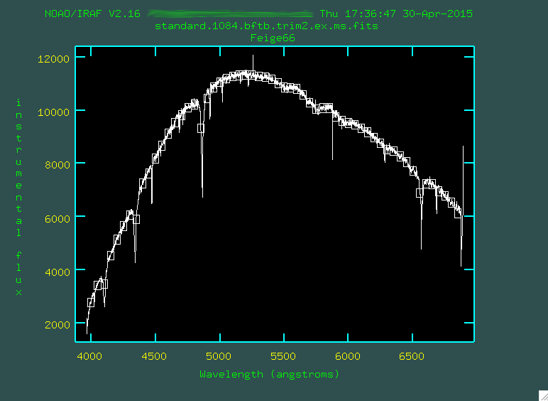 All of the little boxes are defining the flux for this star as compared to the
flux known within IRAF for the star. This looks good (there are no crazy
outlier boxes, where we'd have to delete them (using
All of the little boxes are defining the flux for this star as compared to the
flux known within IRAF for the star. This looks good (there are no crazy
outlier boxes, where we'd have to delete them (using d, naturally).
So, we type q and move on, and the file standard.1084.bftb.trim2.ex.ms.out
will be produced.
In the case where the standard star is not already listed under the stsci
built-in standards, it is quite easy to use your own standard, providing you
provide a standard star calibration file. The calibration file should have
three columns: wavelengths (in Angstroms), calibration magnitudes (in AB
magnitudes), and bandpass widths (also in Angstroms). Many of these files are
available for a variety of standard stars on the
ESO standards
site. Download the appropriate file to the working directory. You may have to
rename the file after the standard star. Then you'll want to change the
caldir:
(caldir = ) Directory containing calibration data
If you type two quotation marks in any parameter line, you'll put in a null
value, which indicates that you want to use a file in your current directory.
Then, when you are asked for the star name in the calibration list, give the name
of the standard star that corresponds to the file you downloaded.
For example, if you want to use the standard star HD93521 for the file
standard.XXXX.bftb.trim.ex.ms.fits, I can go find
the
ESO site for the standard, and download
the magnitudes file
to the working directory. I'd rename the file to "hd93521.dat," and then I'd
run standard:
  standard.XXXX.bftb.trim.ex.ms(1): HD93521
  # STANDARD: Observatory parameters for Michigan-Dartmouth-MIT Observatory
  #       latitude = 31:57.0
  Star name in calibration list (hd93521):
  standard.1077.bftb.trim.ex.ms[1]: Edit bandpasses? (no|yes|NO|YES|NO!|YES!) (yes):
And from here, everything would work out the same way as was done above.
Now, we can run the next step, which is sensfunc:
  PACKAGE = longslit
     TASK = sensfunc

  standard= standard.1084.bftb.trim2.ex.ms.out  Input standard star data file (from STANDARD)
  sensitiv=                 sens  Output root sensitivity function imagename
  (apertur=                     ) Aperture selection list
  (ignorea=                  yes) Ignore apertures and make one sensitivity function?
  (logfile=              logfile) Output log for statistics information
  (extinct= onedstds$kpnoextinct.dat) Extinction file
  (newexti=          extinct.dat) Output revised extinction file
  (observa=       )_.observatory) Observatory of data
  (functio=              spline3) Fitting function
  (order  =                    5) Order of fit
  (interac=                  yes) Determine sensitivity function interactively?
  (graphs =                   sr) Graphs per frame
  (marks  =       plus cross box) Data mark types (marks deleted added)
  (colors =              2 1 3 4) Colors (lines marks deleted added)
  (cursor =                     ) Graphics cursor input
  (device =             stdgraph) Graphics output device
  answer  =                  yes  (no|yes|NO|YES)
  (mode   =                   ql)
Now, this program is going to take in the out file recently produced,
and it will create a sensitivity function (sens.fits). By running the program,
you are going to fit a sensitivity function to your out file. It will ask
if you want to do this interactively:
  > sensfunc
  Fit aperture 1 interactively? (no|yes|NO|YES) (no|yes|NO|YES) (yes):
Indicate yes. You'll be presented with a window:
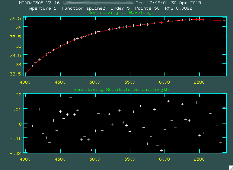 This window shows the sensitivity curve for the instrument based on the
standard star spectrum compared to the internal, correct spectrum for the star.
As you can see, the sensitivity of the OSMOS setup we're using peaks at around
6500 Angstroms. The fit gets worse at the shorter wavelengths, indicated by
the bottom panel residuals, but overall, this fit looks pretty good. If you want
to delete any points from this, you can do so with
This window shows the sensitivity curve for the instrument based on the
standard star spectrum compared to the internal, correct spectrum for the star.
As you can see, the sensitivity of the OSMOS setup we're using peaks at around
6500 Angstroms. The fit gets worse at the shorter wavelengths, indicated by
the bottom panel residuals, but overall, this fit looks pretty good. If you want
to delete any points from this, you can do so with d. When you're
happy with the fit (as I was with the one pictured above), go and
type q to quit out, and the program will produce sens.fits, which is just
the fit to that sensitivity curve you just saw. This will be used to both
correct for chip sensitivity and also to wavelength calibrate.
The final step, then, is to copy this sens.fits file to the folder where
you are planning to flux calibrate your data. I tend to flux
calibrate the data from the folder where I originally ran apextract.
When sens.fits is copied there, you navigate there and run
the task calibrate:
  PACKAGE = longslit
     TASK = calibrate

  input   = j0911.med.ex.ms.fits  Input spectra to calibrate
  output  = j0911.med.ex.flam.ms.fits  Output calibrated spectra
  (extinct=                   no) Apply extinction correction?
  (flux   =                  yes) Apply flux calibration?
  (extinct= onedstds$kpnoextinct.dat) Extinction file
  (observa=       )_.observatory) Observatory of observation
  (ignorea=                  yes) Ignore aperture numbers in flux calibration?
  (sensiti=                 sens) Image root name for sensitivity spectra
  (fnu    =                   no) Create spectra having units of FNU?
  (mode   =                   ql)
And then we can run things like this:
> calibrate
It's important that you don't apply another extinction correction, but you do
apply a flux calibration, and that you have fnu = no, so the final
flux calibrated spectrum comes out in units of ergs/s/cm^2/Angstrom. You can
convert this to an f_nu (erg/s/cm^2/Hz) by either setting fnu = yes,
or, we could use sarith:
> sarith j0911.med.ex.flam.ms.fits fnu "" j0911.med.ex.fnu.ms.fits
The program sarith requires two inputs and an operator
separating them, but when you're running an operation like fnu, or sqrt,
on the spectrum, you just put in "",
which represents "no input", for the second input.
Congrats! Now you have a flux calibrated spectrum! You can apply the same
sens.fits file to your sigma spectrum as well, to flux calibrate it:
  PACKAGE = longslit
     TASK = calibrate

  input   = j0911.med.sig.ex.ms.fits  Input spectra to calibrate
  output  = j0911.med.sig.ex.flam.ms.fits  Output calibrated spectra
  (extinct=                   no) Apply extinction correction?
  (flux   =                  yes) Apply flux calibration?
  (extinct= onedstds$kpnoextinct.dat) Extinction file
  (observa=       )_.observatory) Observatory of observation
  (ignorea=                  yes) Ignore aperture numbers in flux calibration?
  (sensiti=                 sens) Image root name for sensitivity spectra
  (fnu    =                   no) Create spectra having units of FNU?
  (mode   =                   ql)
And now, let's take a look at that spectrum:
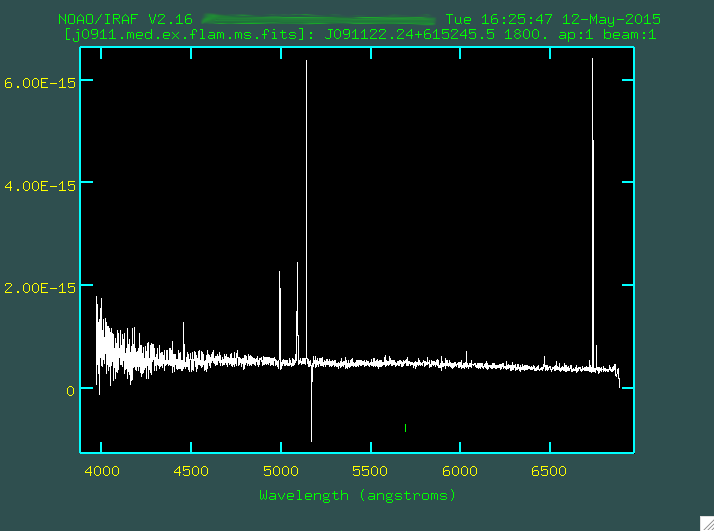 Looking pretty good!
Heliocentric Velocity Correction
The final step is to correct our spectrum for the motion of the sun. We
are going to use an IRAF program called rvcorrect
to calculate the heliocentric correction, and then we'll use
dopcor to actually shift our spectra. First,
rvcorrect requires that you have two
header keywords that, while present in the headers for OSMOS data,
are not in the right form for rvcorrect. First, we
need to get the TIME-OBS from the header, so you can use imheader
to do this:
> imheader j0911.med.ex.flam.ms.fits l+
This resulted in the TIME-OBS value of:
TIME-OBS= '09:19:19.181' / UTC Time at start of obs
Now we can use ccdhedit to edit the header and add in the keyword UT
with this value, along with an EPOCH of 2000:
  > ccdhedit j0911.med.ex.flam.ms.fits UT "09:19:19.181"
  > ccdhedit j0911.med.ex.flam.ms.fits EPOCH "2000"
  > ccdhedit j0911.med.sig.ex.flam.ms.fits UT "09:19:19.181"
  > ccdhedit j0911.med.sig.ex.flam.ms.fits EPOCH "2000"
So, we have to add UT, and EPOCH to the header. Once we've done that, we
can run rvcorrect:
  > rvcorrect images=j0911.med.ex.flam.ms.fits

  # RVCORRECT: Observatory parameters for Michigan-Dartmouth-MIT Observatory
  #       latitude = 31:57.0
  #       longitude = 111:37.0
  #       altitude = 1938.5
  ##   HJD          VOBS   VHELIO     VLSR   VDIURNAL   VLUNAR  VANNUAL   VSOLAR
  2457043.89255     0.00    -0.71     2.58     -0.033   -0.001   -0.675    3.289
V_helio is what we want, which in this case, is -0.71 km/s. We'll want to
remove this from our spectra, which we do using the iraf command dopcor,
found in noao.twodspec.longslit:
  > dopcor j0911.med.ex.flam.ms.fits j0911.med.exhel.flam.ms.fits 0.71 isvel+
  > dopcor j0911.med.sig.ex.flam.ms.fits j0911.med.sig.exhel.flam.ms.fits 0.71 isvel+
We'll use the the negative of the VHELIO value in order to correct
for the heliocentric motion. We've also applied the same correction to the
extinction corrected, flux calibrated sigma spectrum as well.
And so that's it! We now have reduced, flux calibrated, extinction and heliocentric
velocity spectra, with units of F_lambda vs. Angstrom. Perfect for measuring
emission line fluxes! Good luck!
If you want to measure the seeing at the time of your observations, you're going to want to use one of the acquisition images, preferably an acquisition image taken with 1x1 binning. Often, however, you'll only have an acquisition image taken with 4x4 binning, and while the process is the same, the actual correction from pixel FWHM to seeing is not straightforward, as I'll explain below. So, in the sample data, I've included two images, j0911.1073.fits and j0911.1074.fits. If you display them using IRAF, you can see that they look similar, but one is at 1x1 binning (1073) and the other is at 4x4 binning (1074):
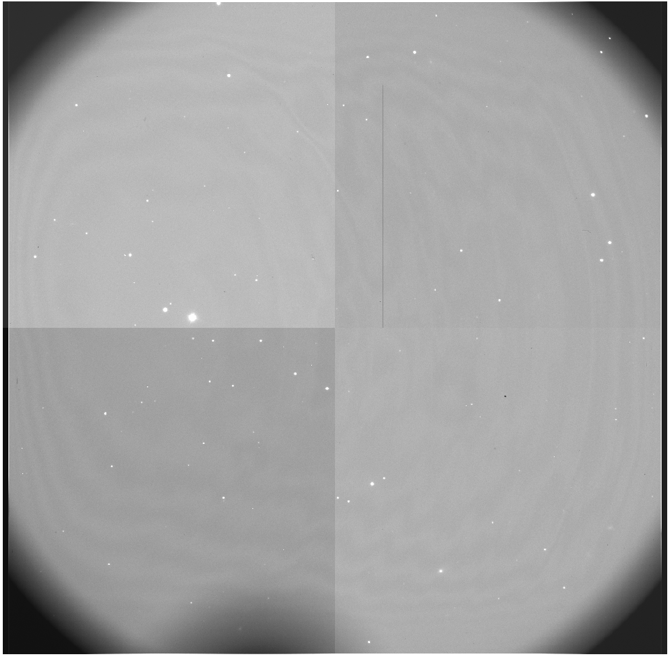
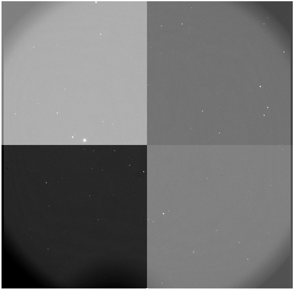 The first step, of course, is to subtract the bias:
  % perl bias_4k_4x4.pl j0911.1073.fits
  % perl bias_4k.pl j0911.1074.fits
Notice that we've used the bias_4k_4x4.pl on 1073, since it's
binned 4x4. If we tried to use the other program, the size of the image would
be entirely screwed up. Let's look at the results:
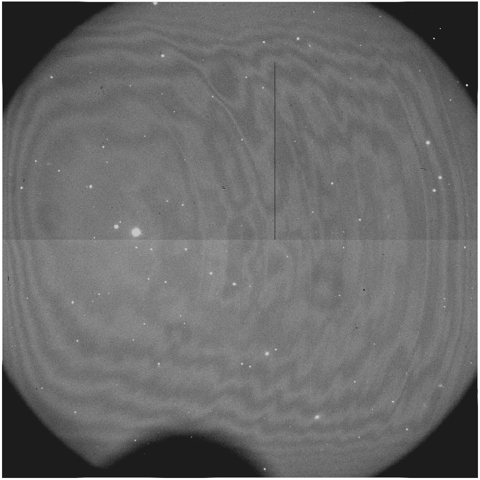
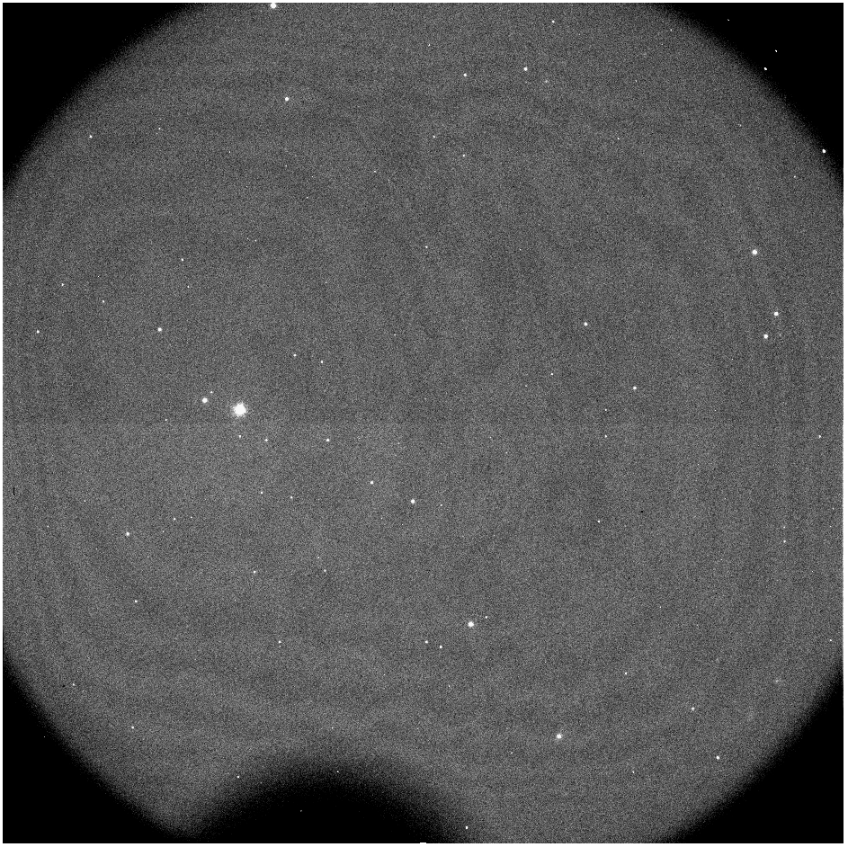 Ah, this is much better. Notice the big shadow on the bottom of the image? That's
the shadow of the guide probe on the image. It's not a big deal for what we're
doing. To measure the seeing, you could use
Ah, this is much better. Notice the big shadow on the bottom of the image? That's
the shadow of the guide probe on the image. It's not a big deal for what we're
doing. To measure the seeing, you could use imexamine, where we
made to change the profile type fittype=gaussian in the rimexam
parameters. However, I like to use psfmeasure in the noao.obsutil
package:
  PACKAGE = obsutil
     TASK = psfmeasure

  images  =    j0911.1074.b.fits  List of images
  (coords =              markall) Object coordinates
  (wcs    =              logical) Coordinate system
  (display=                  yes) Display images?
  (frame  =                    1) Display frame to use

  (level  =                  0.5) Measurement level (fraction or percent)
  (size   =                GFWHM) Size to display
  (beta   =                INDEF) Moffat beta parameter
  (scale  =                   1.) Pixel scale
  (radius =                   5.) Measurement radius (pixels)
  (sbuffer=                   5.) Sky buffer (pixels)
  (swidth =                   5.) Sky width (pixels)
  (saturat=                INDEF) Saturation level
  (ignore_=                   no) Ignore objects with saturated pixels?
  (iterati=                    2) Number of radius adjustment iterations
  (xcenter=                INDEF) X field center (pixels)
  (ycenter=                INDEF) X field center (pixels)
  (logfile=              logfile) Logfile

  (imagecu=                     ) Image cursor input
  (graphcu=                     ) Graphics cursor input
  (mode   =                   ql)
Here, I'm going to start with the image that's using the 1x1 binning, since we
know the raw pixel scale for OSMOS (0.273"/ pixel).
Notice we've specified size=GFWHM, which uses the Gaussian FWHM
values as output. We could also put in the pixel scale here, under the
scale parameter, but let's not, since we're dealing with both
1x1 and 4x4 binned data. If we run psfmeasure now:
  > psfmeasure
  List of images (j0911.1074.b.fits):
It will prompt you to provide a list of images, which you already
specified in the parameters, so just press enter with the one image you've
given it.
  z1=59.50297 z2=173.8004
  ** Select stars to measure with 'm' and finish with 'q'.
  ** Additional options are '?', 'g', and :show.
The program will then display the image in ds9, and your cursor will
change to a blinking annulus. Your job is to select stars in the image by
hovering over them with the mouse and pressing m, and then,
when you're done selecting stars, you'll press q.
When you select stars for this process, don't use the bright stars
with diffraction spikes, since they're most likely saturated. Choose stars
across the image, and make sure they're stars and not faint oblong galaxies.
Once you've picked 10+ stars, press q. A box will show up:
 The center shows the positions of all of the stars that you chose across
the image. Above that is a graph showing the ellipticity of all of the stars
as a function of column. To the right is a graph showing the ellipticity of
the stars as a function of row. The bottom graph is the Gaussian FWHM as a
function of column, and to the left is the Gaussian FWHM as a function of row.
With these graphs, you can see if there is any pattern to the psf as a function
of position across the image. You can go and delete any weird outliers, as
well, in this, by hovering over them and typing
The center shows the positions of all of the stars that you chose across
the image. Above that is a graph showing the ellipticity of all of the stars
as a function of column. To the right is a graph showing the ellipticity of
the stars as a function of row. The bottom graph is the Gaussian FWHM as a
function of column, and to the left is the Gaussian FWHM as a function of row.
With these graphs, you can see if there is any pattern to the psf as a function
of position across the image. You can go and delete any weird outliers, as
well, in this, by hovering over them and typing d. I went and
deleted some of the stars that were near the edges of the images, since they're
not super representative of the seeing, as there are edge effects on the instrument:
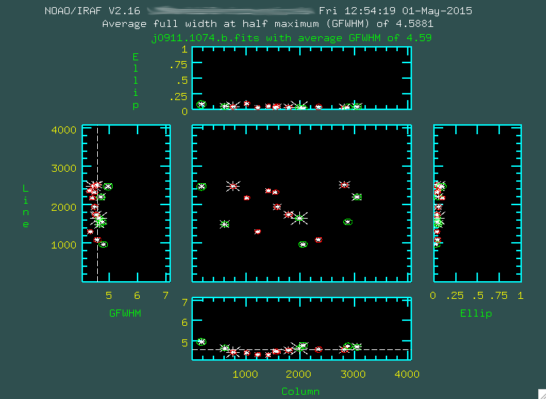 When you're done with that, press
 q again, and it will spit out
the parameters to the screen:
  NOAO/IRAF V2.16 yourusername@yourcomputer Fri 13:01:00 01-May-2015

            Image  Column    Line     Mag   GFWHM   Ellip      PA SAT
  j0911.1074.b.fi  759.61 2484.20    0.35   4.447    0.04     -76
                  1011.06 2181.30    2.66   4.417    0.10      46
                  1573.43 1949.91    1.70   4.485    0.05       5
                  1412.40 2360.36    2.26   4.317    0.05      30
                  1544.10 2328.23    2.64   4.485    0.04      53
                  2819.05 2511.42    1.04   4.577    0.03     -22
                  3056.40 2201.61    1.13   4.704    0.05     -62
                  2883.66 1555.64    2.80   4.753    0.04      21
                  2338.76 1094.15    2.66   4.585    0.04     -20
                  1984.18 1653.61    0.00   4.637    0.04      17
                  1786.18 1744.41    1.33   4.539    0.03      20
                  2050.09  974.17    2.30   4.795    0.02     -52
                   170.12 2474.16    1.72   4.956    0.09     -70
                   604.96 1496.68    1.15   4.665    0.05     -80
                  1218.22 1312.87    2.35   4.339    0.04      21

    Average full width at half maximum (GFWHM) of 4.5881
Here, you want to look at the FWHM of all of the stars, and see if there are
any outliers you missed, but it looks good here. Then you can use the average
to calculate the seeing:
  seeing = <FWHM> * plate scale
  seeing = 4.5881 pixels * 0.273"/pixel
  seeing = 1.3"
So, the seeing for this observation is about 1.3". Now, there's a lesson we
can learn if we try to do this for j0911.1073.b.png as well, and compare:
  > psfmeasure
  List of images (j0911.1074.b.fits): j0911.1073.b.fits
  z1=1457.494 z2=2148.868
  ** Select stars to measure with 'm' and finish with 'q'.
  ** Additional options are '?', 'g', and :show.
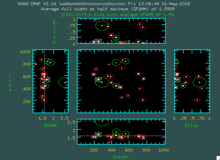 -->
-->
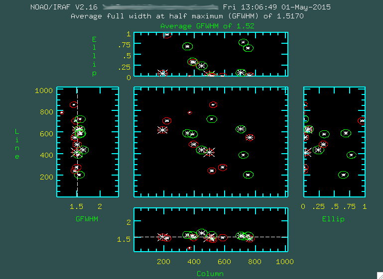
  NOAO/IRAF V2.16 yourusername@yourcomputer Fri 13:08:31 01-May-2015

            Image  Column    Line     Mag   GFWHM   Ellip      PA SAT
  j0911.1073.b.fi  353.25  590.66    2.15   1.579    0.68     -24
                   386.19  582.62    2.57   1.564    0.33     -73
                   393.46  488.12    1.66   1.504    0.32      66
                   446.61  436.70    1.28   1.629    0.24      27
                   496.17  414.08    0.00   1.494    0.03      10
                   190.04  621.62    0.29   1.512    0.06     -10
                   704.84  628.46    0.99   1.559    0.08     -76
                   764.24  551.02    1.14   1.461    0.01     -21
                   721.00  389.62    2.82   1.524    0.77      -3
                   584.71  274.30    2.67   1.497    0.00       0
                   512.55  244.32    2.39   1.457    0.00       0
                   753.34  205.98    2.66   1.555    0.64     -85
                   512.51  721.59    3.17   1.570    0.00       0
                   521.82  854.79    3.35   1.435    0.00       0
                   368.26  781.44    4.58   1.184    0.00       0
                   217.30  706.36    2.43   1.480    0.95       0

    Average full width at half maximum (GFWHM) of 1.5170
Notice that if we naively went with a plate scale of 4*.273"/pixel = 1.092"/pixel:
  seeing = <FWHM> * plate scale
  seeing = 1.5170 pixels * 1.092"/pixel
  seeing = 1.7"
We'd get a much higher seeing! So, obviously, the measured FWHM is affected by the
binning. We can more easily see this by comparing the FWHM of the same star from both images:
            Image  Column    Line     Mag   GFWHM   Ellip      PA SAT
  j0911.1074.b.fi  759.61 2484.20    0.35   4.447    0.04     -76
  j0911.1073.b.fi  190.04  621.62    0.29   1.512    0.06     -10
Again, we'd expect that the FWHM for j0911.1073.b.fits, being a 4x4 binning, should be:
  FWHM = 1.092"/pixel * 1.512 pixels
  FWHM = 1.65"
When, in j0911.1074.b.fits we measure it as:
  FWHM = 0.273"/pixel * 4.447 pixels
  FWHM = 1.21"
So, what's going on here? Well, it turns out that when we bin our data, we
end up "undersampling" the stars in the image. There are not enough pixels
across a given star to accurately sample the radial profile of the star as
it falls off to fit a Gaussian. This is an aspect of Nyquist Theory, as applied
to CCDs, and you can read more
about this here. What this means is that you really should only measure
seeing from 1x1 binned data, or at least data that is well sampled! Otherwise,
you'll end up with too high of seeing estimates, which is not good if you are
trying to understand how the seeing effects your observational data.
OK! So, good luck!