SALT RSS Long-slit Data Reduction
Before We Begin
This page is designed to walk you through reducing the data provided from the SALT pipeline (the "product" data) into wavelength calibrated spectra. Due to the nature of the SALT telescope, absolute flux calibration is not possible. This guide supposes you have science images and an arc lamp image. I will also describe how you could use the flat fields and a standard star observation, as well.
We're going to run the reduction sequence on some sample data from May 18th, 2015, which I have in a folder called "2015-1-SCI-052.20150518". Your data may be found in a similarly named folder. The object we'll be looking at is the quasar candidate SDSS J135925.18-010451.1, which is at an unknown redshift.
First, it's always important to look at the Astronomer's Log (which is found in the /doc folder). Here are the relevant lines to the data we will be reducing:
  20:50 Point
    Block ID: 33326
    Priority: 2
    Proposal: 2015-1-SCI-052
    Target:   J135925.18-010451.1
    PI:       Hickox

  * 20:53 Track Start

  * 21:34
    External seeing is 1.9"
    S10 - field view
    Internal seeing is 2"-2.5"
    S11 - slit view
    P32-34 - 800s, GR900, 1.5" slit
    P35 - 3s, Xe
You can see that they took an image of the field, then an image of the slit, and then took three spectra with the GR900 grating, and a 1.5" slit. Finally, they took a 3 second Xenon arc lamp. For the purposes of this observation, we're also going to use a series of flats taken with the same configuration, but only as an optional step.
And then, let's see if this is true in the Observation Sequence:
The science exposures were:
  P0027 18:47:36 FLAT                  2015-1-SCI-067  2.19 2x4  FS SPN PC03850  PG0900  15.88  31.65 PL0200N001
  P0028 18:47:51 FLAT                  2015-1-SCI-067  2.19 2x4  FS SPN PC03850  PG0900  15.88  31.65 PL0200N001
  P0029 18:48:06 FLAT                  2015-1-SCI-067  2.19 2x4  FS SPN PC03850  PG0900  15.88  31.65 PL0200N001
  P0030 18:48:22 FLAT                  2015-1-SCI-067  2.19 2x4  FS SPN PC03850  PG0900  15.88  31.65 PL0200N001
  P0031 18:48:37 FLAT                  2015-1-SCI-067  2.19 2x4  FS SPN PC03850  PG0900  15.88  31.65 PL0200N001
  P0032 19:00:37 J135925.18-010451.1   2015-1-SCI-052 800.20 2x4  FS SPN PC03850  PG0900  15.88  31.66 PL0150N001
  P0033 19:14:11 J135925.18-010451.1   2015-1-SCI-052 800.20 2x4  FS SPN PC03850  PG0900  15.88  31.66 PL0150N001
  P0034 19:27:44 J135925.18-010451.1   2015-1-SCI-052 800.20 2x4  FS SPN PC03850  PG0900  15.88  31.66 PL0150N001
  P0035 19:42:16 ARC                   2015-1-SCI-052  3.19 2x4  FS SPN PC03850  PG0900  15.88  31.66 PL0150N001
Correct! If we want to look at these images, we'd could do this...
> displ mbxgpP201505180032.fits[sci,1] 1 fill+
...because these images have fits extensions. There are no other extensions
in these images, so this can be annoying. Step one will be to put things
into a format that's easier to view/analyze. Also, take a look at all of the
images in the set!
I've copied my raw data over to a folder that I tend to call "raw_data", and I generally run the reduction in a folder just above raw_data.
Getting the Data Into a Readable Format
Since the images are in an extension format, our first step is to
use imcopy to put the images into a format
that makes the reduction easier. Notice that I am renaming the files
after the object being targeted.
So, in IRAF, we can run things here:
  > imcopy raw_data/mbxgpP201505180032.fits[sci,1] J135925.sci.32.fits
  > imcopy raw_data/mbxgpP201505180033.fits[sci,1] J135925.sci.33.fits
  > imcopy raw_data/mbxgpP201505180034.fits[sci,1] J135925.sci.34.fits
  > imcopy raw_data/mbxgpP201505180035.fits[sci,1] J135925.arc.35.fits
  > imcopy raw_data/mbxgpP201505180027.fits[sci,1] J135925.flat.27.fits
  > imcopy raw_data/mbxgpP201505180028.fits[sci,1] J135925.flat.28.fits
  > imcopy raw_data/mbxgpP201505180029.fits[sci,1] J135925.flat.29.fits
  > imcopy raw_data/mbxgpP201505180030.fits[sci,1] J135925.flat.30.fits
  > imcopy raw_data/mbxgpP201505180031.fits[sci,1] J135925.flat.31.fits
Now, we've got all of the data we care about in one place, in a format where we don't have to specify the fits extension.
Imcombine The Flats (Optional)
We are going to want to combine our flat images. Let's start by making lists:
> ls *.flat.*.fits > flat.list
And now, let's run imcombine with these parameters:
  > imcombine @flat.list flat.med.fits combine=median reject=none scale=mean

  Jun 12 16:54: IMCOMBINE
    combine = median, scale = mean, zero = none, weight = none
    blank = 0.
                  Images     Mean  Scale
        J135925.flat.27.fits  33999.  1.000
        J135925.flat.28.fits  33681.  1.009
        J135925.flat.29.fits  33503.  1.015
        J135925.flat.30.fits  33427.  1.017
        J135925.flat.31.fits  33395.  1.018

    Output image = flat.med.fits, ncombine = 5
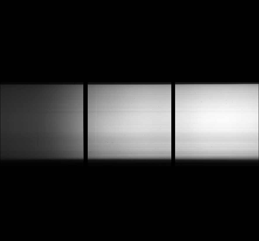
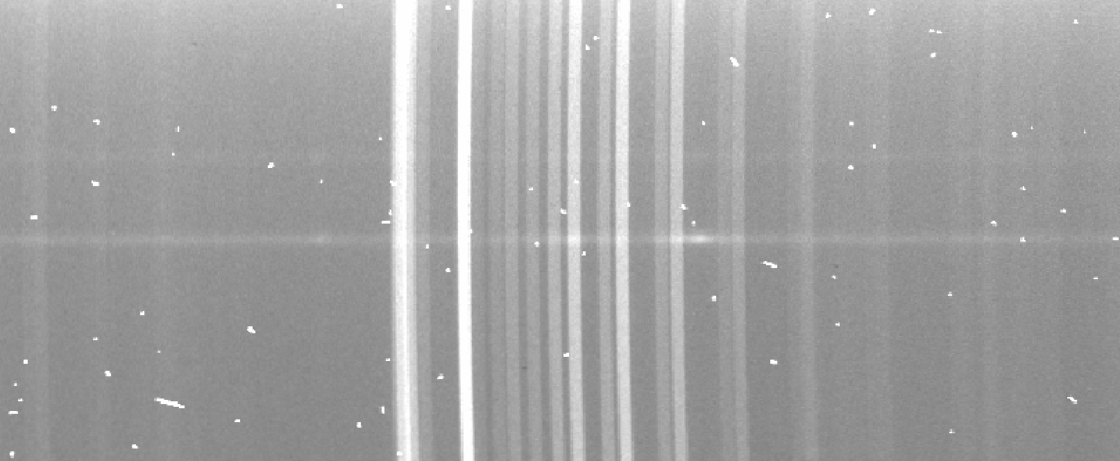
Notice that we're using a median combine, in order to remove the cosmic rays, and we're scaling by the mean so that this makes the median combination make sense. Take a look at the resulting image. It should look something like this:
Make The Illumination Flat (Optional)
We are going to need to take our newly created median flat, and make an
illumination flat for the purposes of dividing by the flat field. We'll need
to use the iraf task mkillumflat, found in the noao.imred.ccdred
packages.
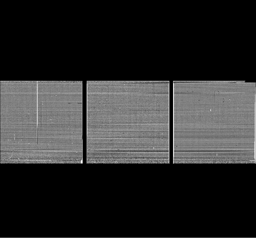
> mkillumflat input=flat.med.fits output=flat.med.i.fits ccdtype="" xboxmin=3 yboxmin=3 xboxmax=5 yboxmax=5
Take a look at the result. If it looks all right, we'll move on. You can see in this example that there's a feature near the bottom right, but as it's nowhere near the central trace that we care about, it's not a huge deal.
Flat Reduce Each Science Image (Optional)
So, we'll want to first normalize our flat, so that the counts for the flat-reduced science image aren't crazy. This step is not super critical, but I like to do it nonetheless. First, let's find the average count level for the newly created illumination flat:
  > iterstat flat.med.i.fits
  flat.med.i.fits: mean=33203.24  rms=9292.192  npix=3253446  median=33888.95  mode=33908.7
  flat.med.i.fits: mean=32846.37  rms=6353.208  npix=3242252  median=33872.55  mode=33927.16
  flat.med.i.fits: mean=33908.38  rms=1611.746  npix=3132767  median=33884.14  mode=33885.15
  flat.med.i.fits: mean=33908.94  rms=565.0006  npix=3109929  median=33885.49  mode=33886.98
  flat.med.i.fits: mean=33892.59  rms=282.4241  npix=3079090  median=33891.34  mode=33893.97
  flat.med.i.fits: mean=33888.82  rms=230.5504  npix=3060018  median=33885.73  mode=33891.01
  flat.med.i.fits: mean=33888.82  rms=221.0607  npix=3051680  median=33888.25  mode=33893.64
  flat.med.i.fits: mean=33888.83  rms=219.2065  npix=3049646  median=33882.18  mode=33887.51
  flat.med.i.fits: mean=33888.82  rms=218.8493  npix=3049236  median=33889.67  mode=33894.88
  flat.med.i.fits: mean=33888.81  rms=218.763  npix=3049136  median=33891.02  mode=33896.19
This is just running an iterative statistics program on the image, and
the most important number I've put in bold. This is the mean for the image. We
can use imarith to divide by this value:
> imarith flat.med.i.fits / 33888.81 flat.med.i.norm.fits
And now, we can use imarith to divide our science target by the flat:
  > imarith J135925.sci.32.fits / flat.med.i.norm.fits J135925.sci.32.f.fits
  > imarith J135925.sci.33.fits / flat.med.i.norm.fits J135925.sci.33.f.fits
  > imarith J135925.sci.34.fits / flat.med.i.norm.fits J135925.sci.34.f.fits
As always, take a look at the resulting flat reduced science image. It should look pretty good.
Note, for the remainder of this guide, I won't be using the flat reduced data. If you want to use the flats, note that there is a *.f.* throughout in the file names, and you should probably keep using this convention.
Trimming The Data
For our purposes here, we don't really care much about the spectrum outside of a certain wavelength range. We also don't care much about a lot of the portion of the image well above or below the spectrum. So, we should use imcopy to trim out only the portion we care about. We will have to do this to both our image and to the arc lamp, in the same way, or else everything won't line up correctly.
To that end, we have to make sure that we target the central portion of the SALT 2D spectrum, so if you open up one of the science images in ds9, you should look to see where the central trace is:
Here, notice that there are some faint horizontal traces. I assume that the brightest one at the center is the object we care about, and we can check this, providing the SALT observers have given us an image of the sky taken as they were acquiring the target. You can check this in the product folder. To find the sky image for this particular observation, I looked at the observation log and saw these lines:
    S201505180010 J135925.18-0 1          -01:04:51 SCM NO SDSSi-S 4x4 FA FA         0.00   0.00   10.0 18:54:31 2015-1-SCI-052  Hickox
    S201505180011 J135925.18-0 1          -01:04:51 SCM NO SDSSi-S 4x4 FA FA         0.00   0.00    2.0 18:59:57 2015-1-SCI-052  Hickox
    P201505180032 J135925.18-0 1          -01:04:51 RSS IM PC03850 2x4 FA SL PG0900 15.88  31.66  800.2 19:00:37 2015-1-SCI-052  Hickox
    P201505180033 J135925.18-0 1          -01:04:51 RSS IM PC03850 2x4 FA SL PG0900 15.88  31.66  800.2 19:14:11 2015-1-SCI-052  Hickox
    P201505180034 J135925.18-0 1          -01:04:51 RSS IM PC03850 2x4 FA SL PG0900 15.88  31.66  800.2 19:27:44 2015-1-SCI-052  Hickox
    P201505180035 ARC          1          -01:04:51 RSS IM PC03850 2x4 FA SL PG0900 15.88  31.66    3.2 19:42:16 2015-1-SCI-052  Hickox
And I noticed that the file S201505180010 is an image using
"SCAM," the slit camera. So, let's open it up in ds9:
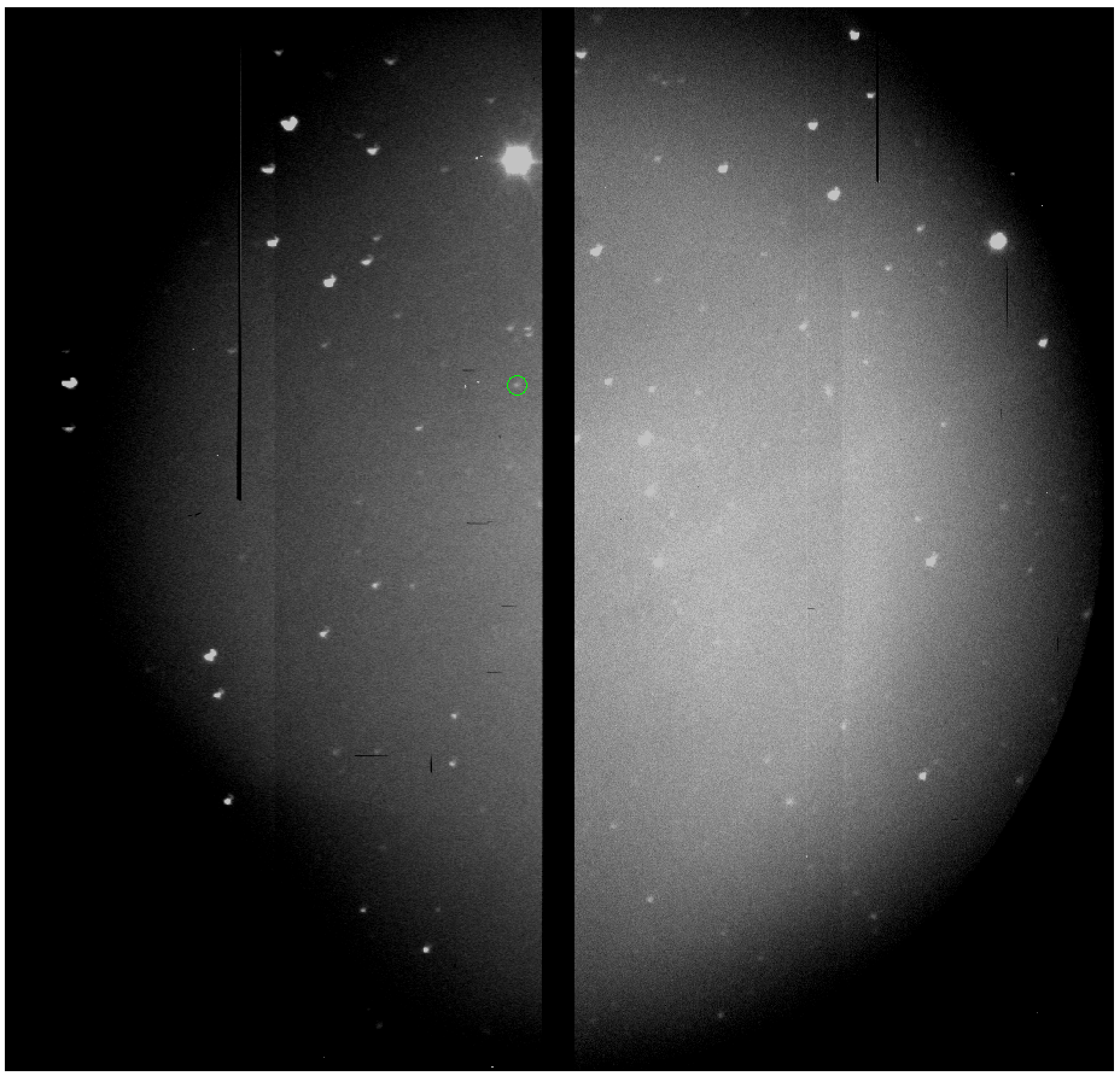
I also, at this point, open up the pdf of the finder chart for SDSS J135925.18-010451.1, or I can go and look up what the field that has our object:
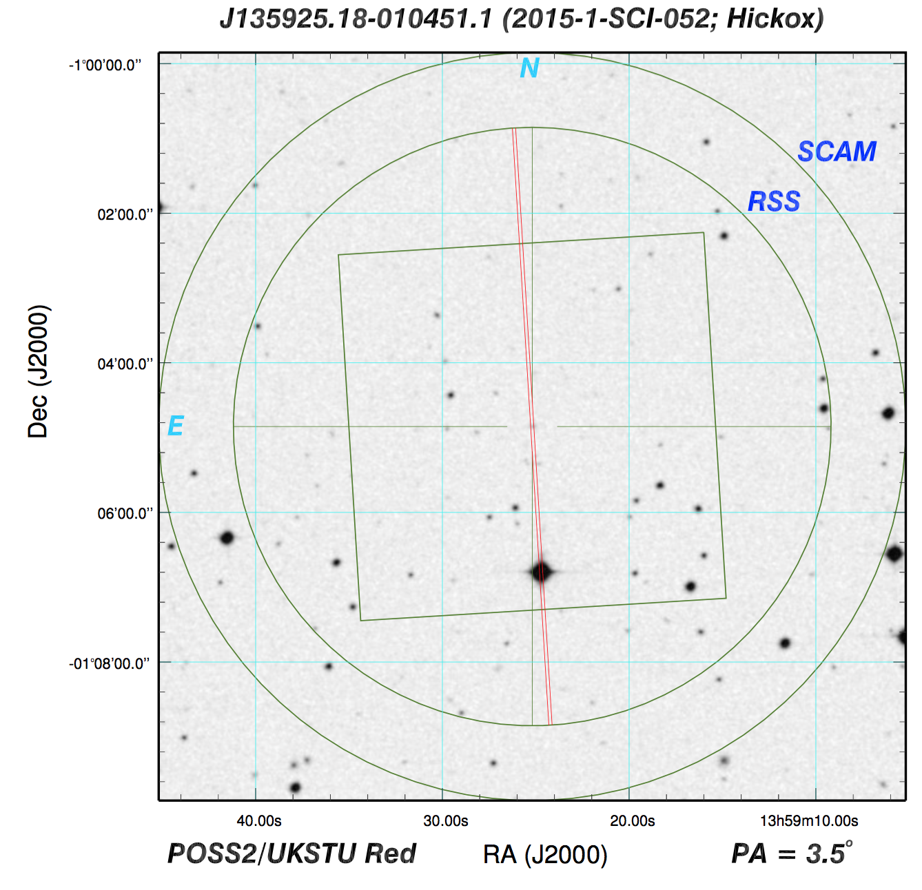
Now, the game becomes trying to figure out which object in the SCAM image corresponds to our target. I've circled it above, but make sure that you can figure this out on your own, which requires rotating the finder chart around a bit. From here, we can see that there is another bright source on the slit, which is very obvious from our science 2D spectrum. We can use these two images to find our target on the 2D image, which is at y=520.
This means we'll want to trim around there, maybe from 420 < y < 620. We'll also want to get the whole slit in the wavelength direction, so let's go from 50 < x < 3160.
  > imcopy J135925.arc.35.fits[50:3160,420:620] J135925.arc.35.trim.fits

  > imcopy J135925.sci.32.fits[50:3160,420:620] J135925.sci.32.trim.fits
  > imcopy J135925.sci.33.fits[50:3160,420:620] J135925.sci.33.trim.fits
  > imcopy J135925.sci.34.fits[50:3160,420:620] J135925.sci.34.trim.fits
Take a look at the resulting images:


Identify
So, now we're going to do the only difficult portion of this reduction
procedure, the part where we identify emission lines in the arc lamp spectrum for
the purposes of wavelength calibration. The way in which this works is that
we use an iraf task called identify, which
first plots the center of the arc image, showing the peaks, and then allows the
user to provide the wavelengths of those peaks. From here, a fit will be performed
between the pixel values and the wavelength values for the peaks near the center
of the image, and you will move on to the task
reidentify.
For this redshift and grating configuration, the SALT astronomers have used the Xenon arc lamp. I know this because in the original product file, I used:
ecl> imhead mbxgpP201505180035.fits[0] l+
And I got a huge dump of information, but the most important information is:
  CCDTYPE = 'ARC               ' / CCD Type
  LAMPID  = 'Xe                ' / name of lamp
  ...
  GRATING = 'PG0900            ' / Commanded grating station
  ...
  GRTILT  =            15.875000 / Commanded grating angle
  ...
  AR-ANGLE=            31.662090 / Articulation angle from incremental encoder
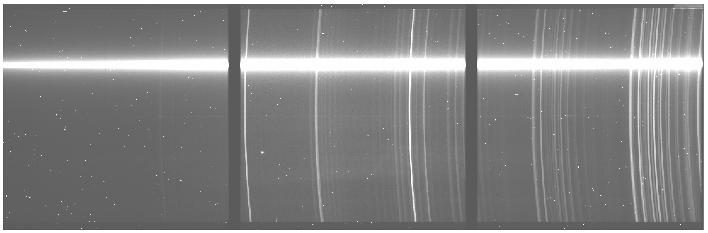
This is a Xenon arc lamp, with the PG0900 grating, at a grating angle of 15.875 and an articulation angle of 31.66. These numbers will help you when you're trying to find what Xenon arc spectrum to look at, and have been chosen to center the spectrum on a specific wavelength. In this case, you're going to want to navigate to the SALT Xenon arc images. The full list of files for various elements can be found here. We'll also want to download the Xenon file "Xe.txt," from the same website. Put that file in the same folder as you're doing your reduction.
Anyway, open up the pdf and navigate to the plot that most closely matches the instrument configuration described in the header, which, for this, looks like Figure 16.
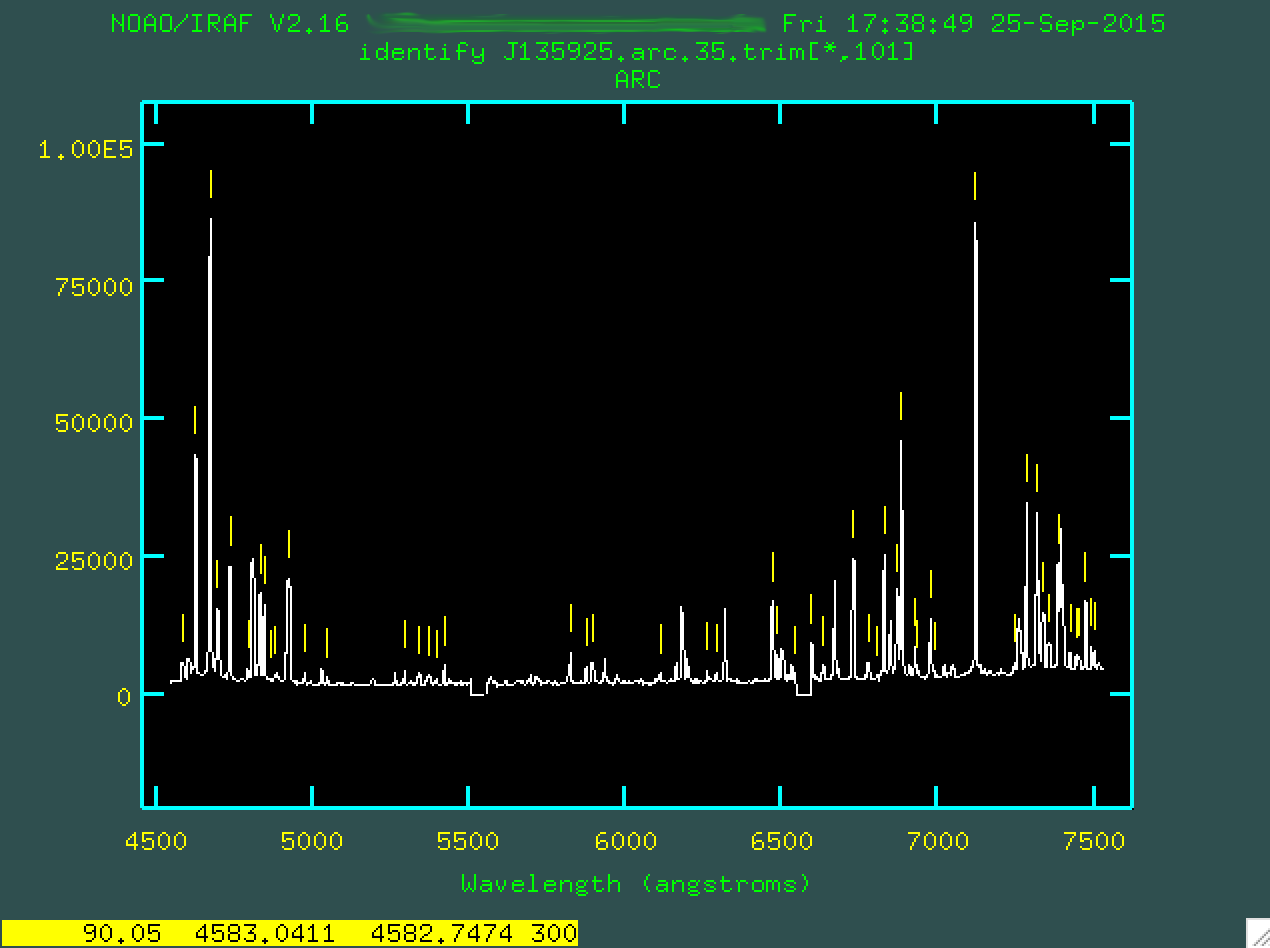
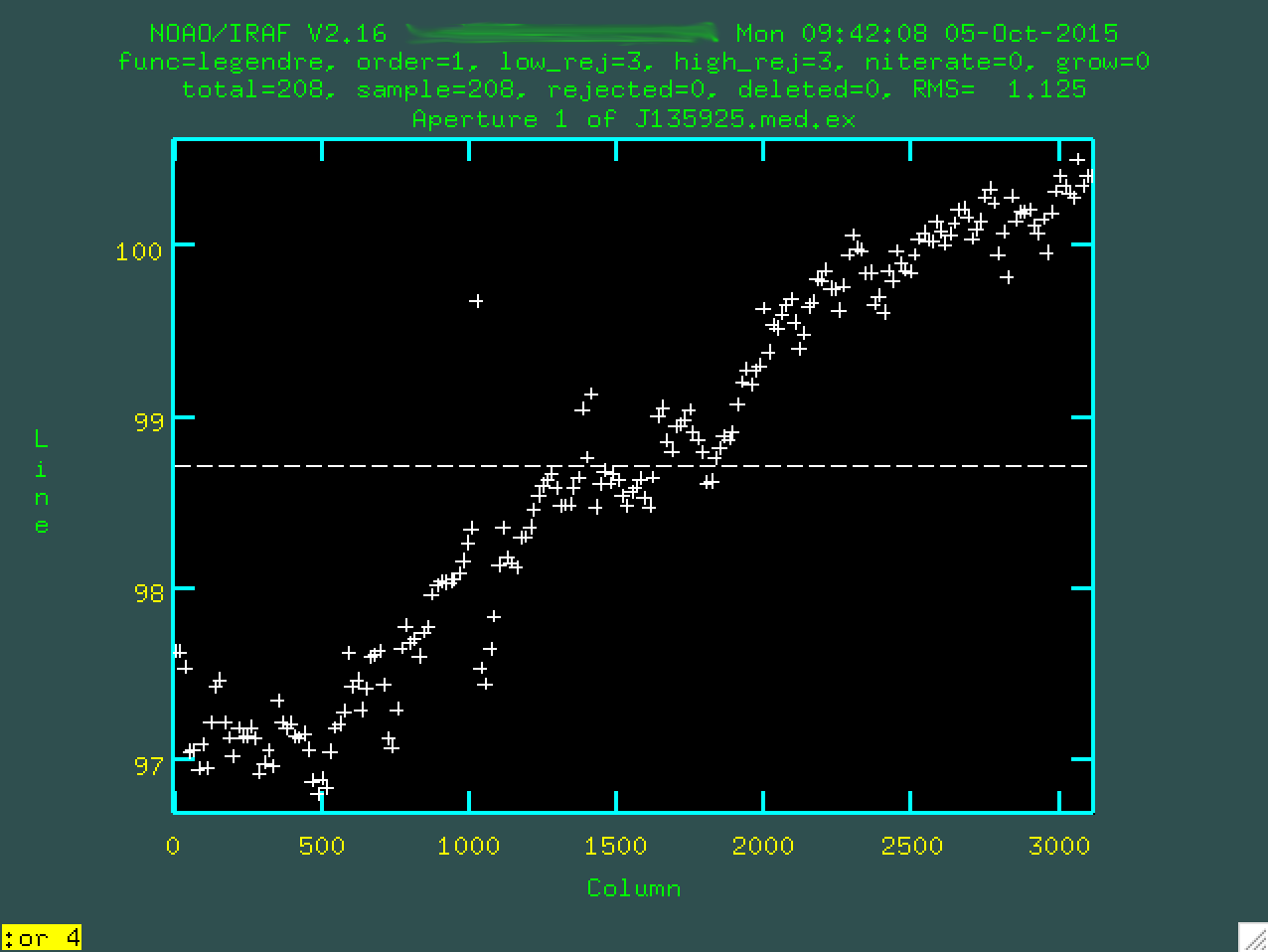
Now, take a deep breath, and run identify on the arc image:
> identify images=J135925.arc.35.trim.fits coordlist=Xe.txt function=chebyshev order=5 fwidth=6. cradius=6
There are a few important things to notice from how we ran identify.
First, we need to make sure that
the coordlist is set to the file that you should have downloaded corresponding
to that particular arc lamp. It's a pain to input the exact-to-the-decimal wavelength
value for each and every line you want to fit, so a coordlist is used. When you
input a wavelength value, identify will go
through the coordinates list and grab the nearest wavelength in the list, which
makes everyone's lives easier. Also, once you input a few correct wavelength values
and create a rough fit, identify can be told to
look through the coordlist and just find the peaks that are closest in rough
wavelength to the lines in the list, which speeds things up considerably.
Secondly, the order for the fit specified here is 5,
but you want to go with the lowest order that produces results you think look
good. For some arc spectra, I have to use order=3 or else
reidentify breaks as such a high order fit ends
up not being well constrained. It's not a huge deal in the grand scheme of
things, but do what you want. Just know that you may have to redo identify
quite a bit, and this is a parameter you can futz with.
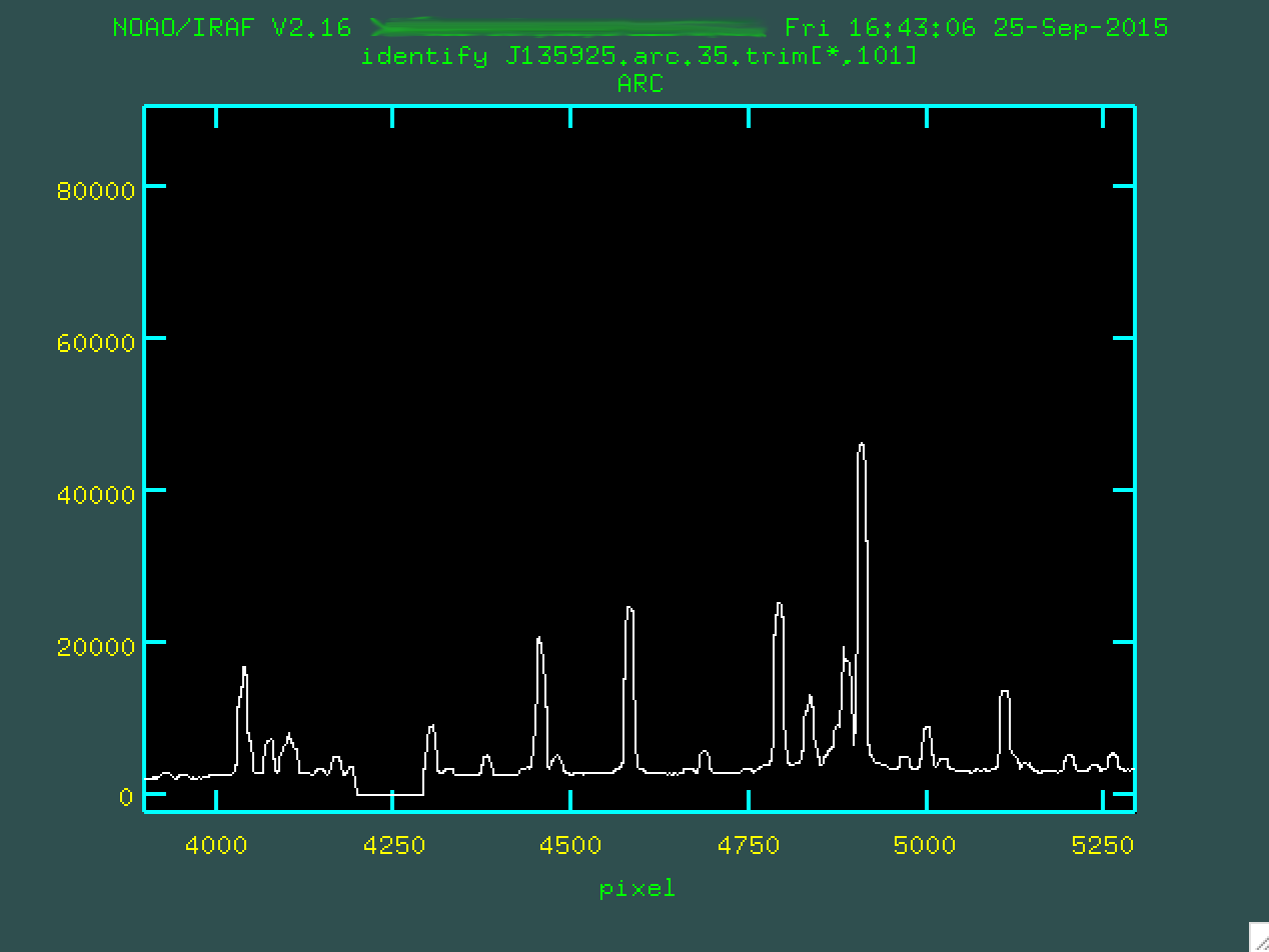
Now, when you run that identify line, you'll
be presented with the spectrum of the emission features from the center of the
image.
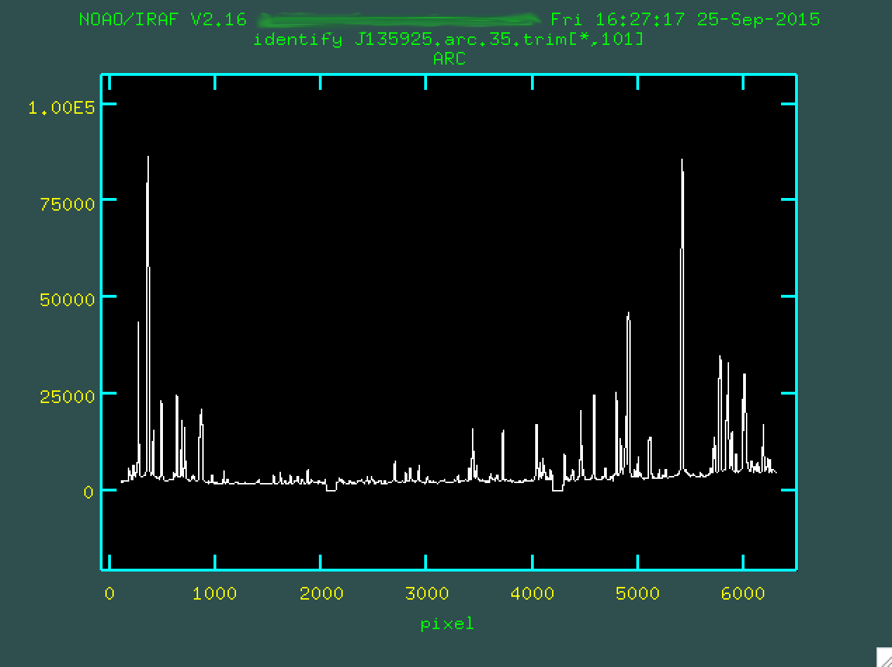
Your job is to go through and identify the lines you see in your sample arc
spectrum in the one you've measured here, and mark them. To do this, you're going
to want to really zoom in on the pdf, and also zoom in on a region of interest
in the arc. To zoom in, you should make sure you've clicked on the pop-up
window that shows the arc spectrum type w (for "window").

At this point, you want to move the mouse to the bottom left of the zoom-in
region that you want, and at that point, type e:

Then go and move the cursor to the top right of the zoom-in region that you want...

...and you should press e again.
You can zoom back out by typing w n and w m, by the
way.
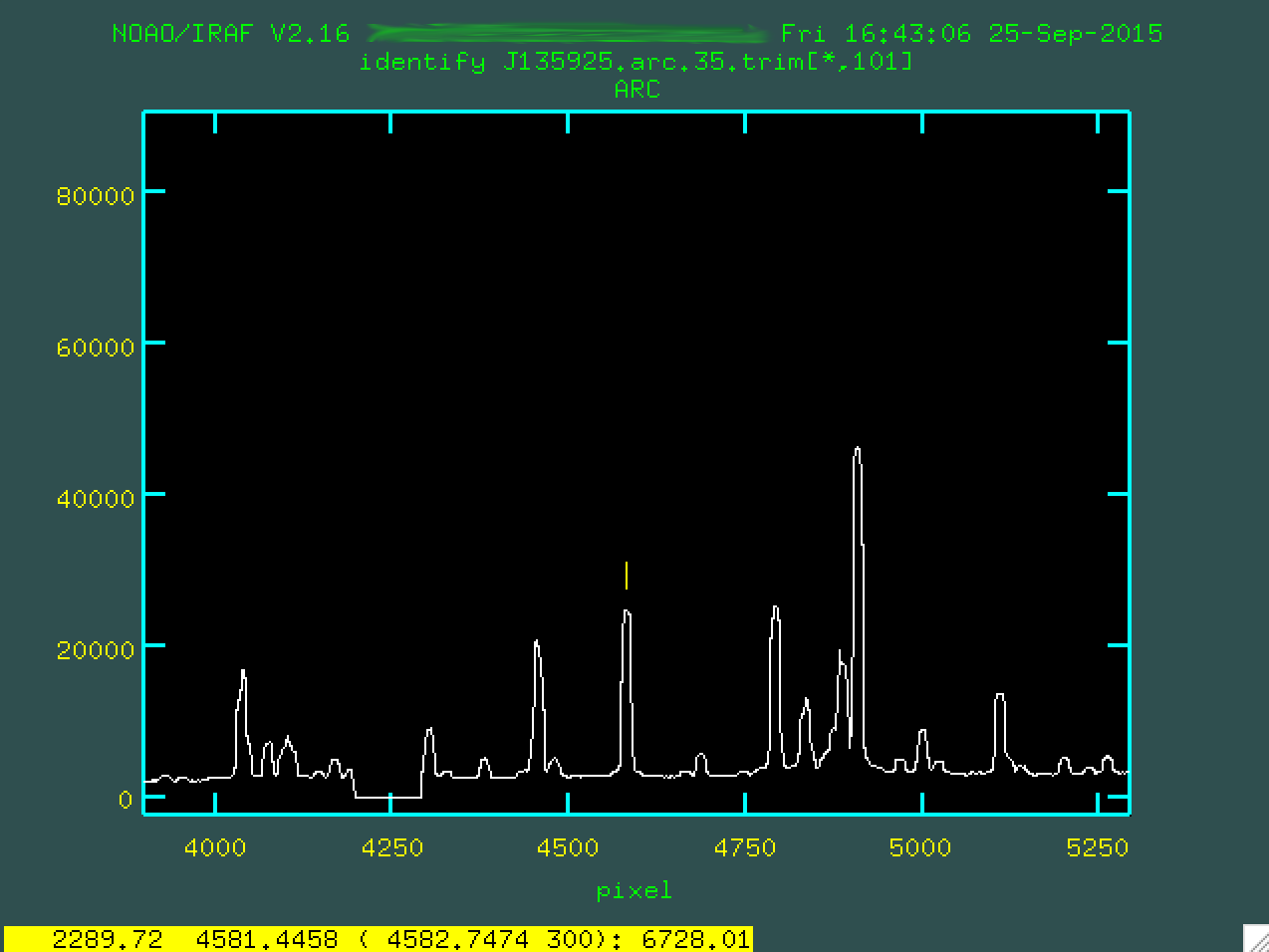
Next, you should line up the cursor on a line you think you know the wavelength
for and press m, and then type in the wavelength of the feature as well as
you know it. So, for instance, looking at the pdf, I've identified the line
below as being at 6728.01 Angstroms. So, I moused over the line, typed m,
and then typed in 6728.01:
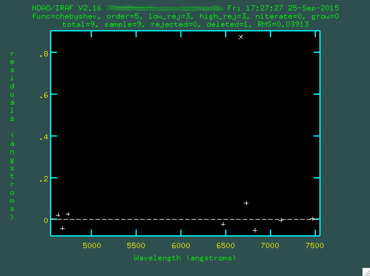
From here, let's mark another three or four lines. We'll want to pin down both sides of the wavelength scale. So, here are the lines I found:
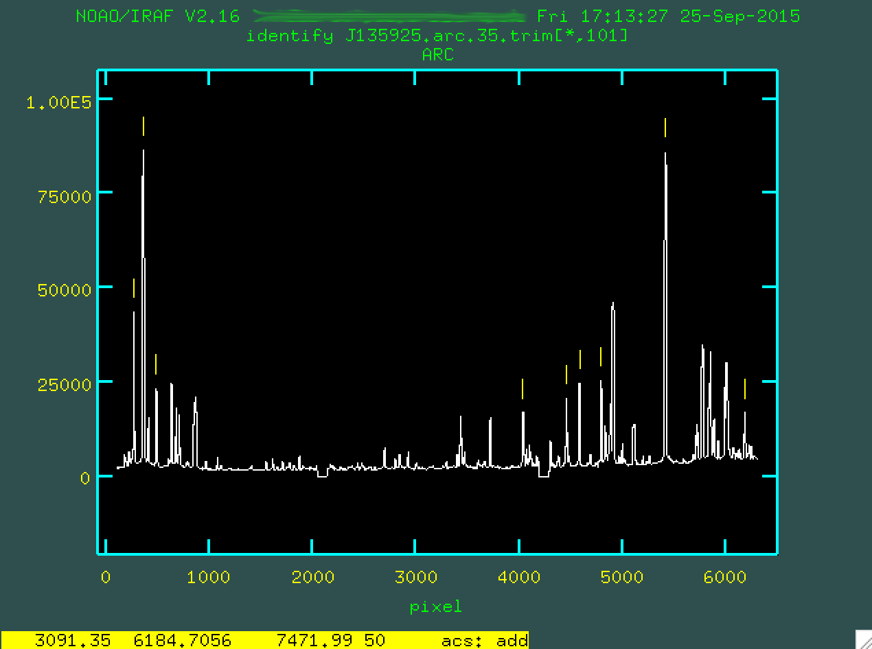
Notice that I have actually identified some lines to the red of what is
shown in Figure 16, like the big strong line on the right side of the image. To
do this, I went down to Figure 17, and found those lines. Simple enough. Now,
from here, you want to make sure that you have the coordinates list ("Xe.txt")
in the folder where you've run identify. At this point, you can
type f to run a preliminary fit on your lines.
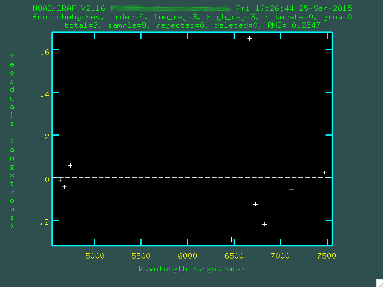
You're looking at the residuals from the fit, ie, the biggest outlier points.
Sometimes, the fit will look ok, potentially. If it does, you can move on. Here, though,
I'm not happy with that crazy outlier point, so I can go and hover over it and
press d to delete it.

And now you can type f to redo the fit.
Now, you can go back to the emission lines, by typing q. Here,
notice that your fit means that the x axis of the plot is wavelength, instead of
pixels. But, we want to refine the fit. You could go and identify every single
line in the same tedious way, but with a preliminary fit and a line list, we can
actually just type l and the program will go and find a bunch of
strong lines and try to figure out what they correspond to (in a dumb way)
in the coordinates list.
Now, type f to fit all of these new lines.
The fit should look ok, but you might have to go through and trim out
poorly fitted points. Line the cursor up over these points and type d to delete
these points.
 Then press
 f to re-fit.

Watch that rms drop!
Eventually, you'll be happy with the fit, and you can type q from the
spectrum (if you type q from the fit, you'll be taken to the spectrum,
remember), and the IRAF window will ask you if you want to write the feasture data
to the database. You can press enter, since often, "yes" is the default. Otherwise,
you can type yes. If you're not happy, and want to redo everything,
type no, of course.
Reidentify
Our next goal is to take our wavelength solution and perform it up and down
across the 2D spectrum. To do this, we're going to want to use the IRAF task
reidentify:
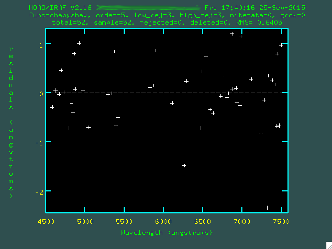
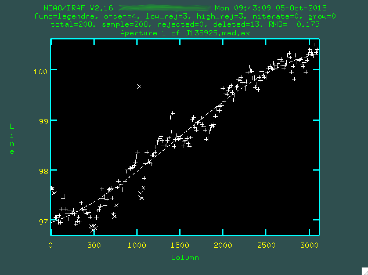
> reidentify reference=J135925.arc.35.trim.fits images=J135925.arc.35.trim.fits interactive=no newaps=yes override=no refit=yes nlost=20 coordlist=Xe.txt verbose=yes > reidentify.log
This will propogate the wavelength solution along the slit, up and down across the image. In the end, you'll get a file ("reidentify.log") that should look like this:
  ecl> cat reidentify.log

  REIDENTIFY: NOAO/IRAF V2.16 XXX@XXX Mon 16:11:12 28-Sep-2015
    Reference image = J135925.arc.35.trim.fits, New image = J135925.arc.35.trim, Refit = yes
            Image Data    Found     Fit Pix Shift  User Shift  Z Shift      RMS
  J135925.arc.35.trim[*,91] 50/50   50/50     0.0328      0.0311  4.77E-6    0.527
  J135925.arc.35.trim[*,81] 50/50   50/50      0.197        0.19  3.41E-5    0.477
  J135925.arc.35.trim[*,71] 50/50   50/50      0.123       0.115  1.68E-5    0.554
  J135925.arc.35.trim[*,61] 48/50   48/48       0.12       0.114  1.80E-5    0.476
  J135925.arc.35.trim[*,51] 48/48   48/48      0.121       0.114  1.79E-5     0.42
  J135925.arc.35.trim[*,41] 48/48   48/48      0.185       0.179  3.04E-5    0.452
  J135925.arc.35.trim[*,31] 48/48   48/48      0.157       0.151  2.56E-5    0.528
  ...
And on. Notice that the RMS is about the same as was done along the center of
the slit when you ran identify. Hopefully, if the arc spectral lines
are strong enough, this will be the case.
Fitcoords
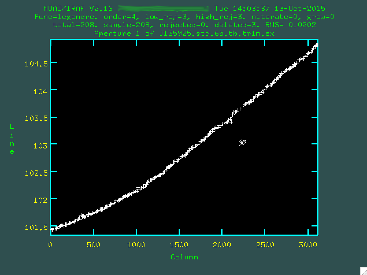
Now, let's create the final 2D wavelength solution that we'll apply to our
actual science image. To do this, we'll use the IRAF task fitcoords,
which also requires some interaction. We'll run it like this:
> fitcoords images=J135925.arc.35.trim interactive=yes combine=no functio=legendre xorder=5 yorder=3
A question will be asked:
Fit J135925.arc.35.trim interactively (yes):
You should probably press enter, since you do want to do this interactively
(in fact, this is why we set interactive=yes, but whatever). More
text will print to the terminal:
  NOAO/IRAF V2.16 XXX@XXX Mon 16:19:39 28-Sep-2015
    Longslit coordinate fit name is J135925.arc.35.trim.
    Longslit database is database.
    Features from images:
      J135925.arc.35.trim
And another window will open up, like when we ran identify:
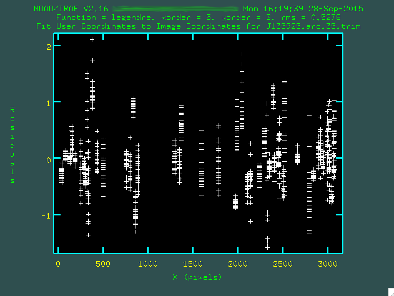
Each one of the bundles of points that you see corresponds to a fitting of
an arc emission line as a function of position up and down along the spatial
direction. The fit will try to go through all of the points, and you can go
and remove outliers in a similar way to how it was done in identify,
by hovering over a point and pressing d. However, instead of just
deleting individual points, you are also given the option to delete all of the
points in the same x, y, or z coordinate. This is kind of a black box-ey
process. I've run this a bunch, and I mostly just make sure that the fit does
not seem to be overly dependent on some outlier points, and then I call it a
day. You can also change the order of the fit using :xor X or
:yor X, where X is the new fit.
For the fit above, I definitely didn't like a few columns of outlying points,
so I deleted them by hovering over one of the points in the column and typing
d and then z. I also deleted some of the individual
outlier points by hovering over them and typing d and then p.
After each deletion, I refit by typing f:
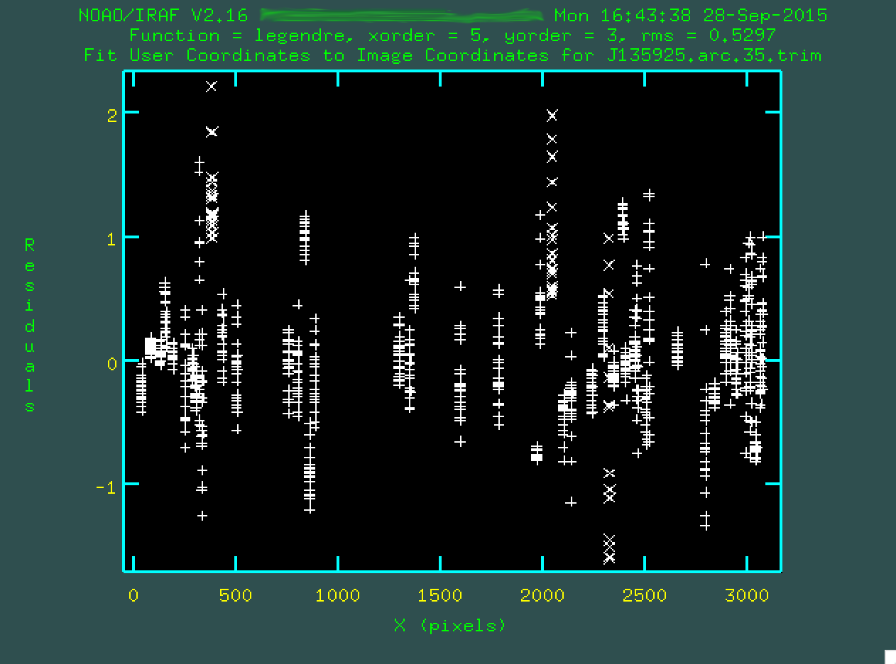
When you're done with the fit, type q, and at this point
fitcoords will print more out to the terminal:
    Map User coordinates for axis 1 using image features:
    Number of feature coordnates = 1036
    Mapping function = legendre
      X order = 5
      Y order = 3
    Fitted coordinates at the corners of the images:
      (1, 1) = 4541.631  (3111, 1) = 7533.752
      (1, 201) = 4542.817  (3111, 201) = 7534.766
  Write coordinate map to the database (yes)?
If you were happy with the run and the fit, press enter,
and it will be recorded to a database file ("database/fcJ135925.arc.35.trim" in
this case).
Cosmic Ray Zapping
Now, we have our wavelength calibration, but we want to run cosmic ray zapping on our data, which is primarily so we can create a bad pixel mask for use when stacking the data. We'll be median stacking the data anyway, and that should get rid of the cosmic rays, but sometimes SALT data will only have two frames, in which case we'll really need to do this.
Similar to what I discuss in my OSMOS data reduction site,
I use a user script xzap to cosmic ray zap. You should navigate
over to that page to install xzap, where I describe how to download
and install the user script. From here, you want to set your xzap
parameters like this:
  inlist  =  J135925.sci.32.trim  Image(s) for cosmic ray cleaning
  outlist = J135925.sci.z.32.trim  Output image(s)
  (zboxsz =                    8) Box size for zapping
  (nsigma =                   9.) Number of sky sigma for zapping threshold
  (nnegsig=                   0.) Number of sky sigma for negative zapping
  (nrings =                    2) Number of pixels to flag as buffer around CRs
  (nobjsig=                   2.) Number of sky sigma for object identification
  (skyfilt=                   15)   Median filter size for local sky evaluation
  (skysubs=                    1)   Block averaging factor before median filtering
  (ngrowob=                    0)   Number of pixels to flag as buffer around objects
  (statsec=  [2164:2297,130:180]) Image section to use for computing sky sigma
  (deletem=                   no) Delete CR mask after execution?
  (cleanpl=                  yes) Delete other working .pl masks after execution?
  (cleanim=                  yes) Delete working .imh images after execution?
  (verbose=                  yes) Verbose output?
  (checkli=                  yes) Check min and max pix values before filtering?
  (zmin   =              -32768.) Minimum data value for fmedian
  (zmax   =               32767.) Minimum data value for fmedian
  (inimgli=                     )
  (outimgl=                     )
  (statlis=                     )
  (mode   =                   ql)
The most important thing for you to change on an object-by-object basis is
the statsec, a region used to compute the nominal background level.
The format of the statsec is [XXX:XXX,YYY:YYY], where XXX:XXX is
the xmin and xmax "image" pixel values, and YYY:YYY is the ymin and ymax "image"
pixels values of a region on the image without any signal from the trace, but
near it. For the object we're examining in the example data, I used
[2164:2297,130:180]. You can also specify the statsec
when you call xzap, and I'll demonstrate that below.
If you run the cosmic ray zapping before transforming your data, you will have to include your mask to be transformed along with the data. If you run cosmic ray zapping after transforming the data, you've moved around some of the cosmic ray flux, which is non-ideal, so always run it beforehand.
Now, let's run xzap like this:
  > xzap J135925.sci.32.trim J135925.sci.32.z.trim statsec=[2164:2297,130:180]
  > xzap J135925.sci.33.trim J135925.sci.33.z.trim statsec=[2164:2297,130:180]
  > xzap J135925.sci.34.trim J135925.sci.34.z.trim statsec=[2164:2297,130:180]
A bunch of text will be written to the screen:
  Working on J135925.sci.32.trim ---ZAP!--> J135925.sci.32.z.trim
       Computing statistics.
  J135925.sci.32.trim[2164:2297,130:180]: mean=216.0499  rms=15.83263  npix=6834  median=215.7164  mode=213.7244
       Median filtering.
       Data minimum = 0.  maximum = 51191.45703125
       Truncating data range 0.  to 32767.
       Masking potential CR events.
       Creating object mask.
       Thresholding image at level 31.58458201
       Growing mask rings around CR hits.
       Replacing CR hits with local median.
  add J135925.sci.32.trim,CRMASK = crmask_J135925.sci.32.trim.pl
  add J135925.sci.32.z.trim,CRMASK = crmask_J135925.sci.32.trim.pl
       Done.
And you should look at the results to see if they look all right.
 Before cosmic ray zapping (J135925.sci.32.trim.fits)
 After cosmic ray zapping (J135925.sci.32.z.trim.fits)
 Cosmic ray mask (crmask_J135925.sci.32.trim.pl)
It's important that the cosmic ray zapping doesn't mask off emission features,
or parts of a bright trace (if your central trace is, indeed super bright). If
that happens, you need to go back and change the sigma values in the
Cosmic ray mask (crmask_J135925.sci.32.trim.pl)
It's important that the cosmic ray zapping doesn't mask off emission features,
or parts of a bright trace (if your central trace is, indeed super bright). If
that happens, you need to go back and change the sigma values in the xzap
procedure and re-run everything. Eventually, you'll get something that looks good.
Now, what's interesting is that even though we produced *.z.trim.fits files, we
won't be using them if we have three or more images, because we can use median
combining at the end. If you just have two images in a set, you'll have to use
these cosmic ray zapped images going on, because you can't take a median with
only two images.
Transform
And next, we want to transform our images, using, appropriately, the IRAF task
transform. Note that we also transform our bad pixel masks, as well,
and create some files with "t" in the name:
  > transform input=J135925.sci.32.trim output=J135925.sci.32.t.trim minput=crmask_J135925.sci.32.trim.pl moutput=crmask_J135925.sci.32.t.trim.pl fitnames=J135925.arc.35.trim interptype=linear flux=yes blank=INDEF x1=INDEF x2=INDEF dx=INDEF y1=INDEF y2=INDEF dy=INDEF
  > transform input=J135925.sci.33.trim output=J135925.sci.33.t.trim minput=crmask_J135925.sci.33.trim.pl moutput=crmask_J135925.sci.33.t.trim.pl fitnames=J135925.arc.35.trim interptype=linear flux=yes blank=INDEF x1=INDEF x2=INDEF dx=INDEF y1=INDEF y2=INDEF dy=INDEF
  > transform input=J135925.sci.34.trim output=J135925.sci.34.t.trim minput=crmask_J135925.sci.34.trim.pl moutput=crmask_J135925.sci.34.t.trim.pl fitnames=J135925.arc.35.trim interptype=linear flux=yes blank=INDEF x1=INDEF x2=INDEF dx=INDEF y1=INDEF y2=INDEF dy=INDEF
When you run transform, some text will print to the screen,
describing the output of the transformation:
  NOAO/IRAF V2.16 XXX@XXX Tue 10:14:49 29-Sep-2015
    Transform J135925.sci.32.trim to J135925.sci.32.t.trim.
    Transform mask crmask_j135925.sci.32.trim.pl to crmask_j135925.sci.32.t.trim.pl.
    Conserve flux per pixel.
    User coordinate transformations:
      J135925.arc.35.trim
    Interpolation is linear.
    Using edge extension for out of bounds pixel values.
    Output coordinate parameters are:
      x1 =      4542., x2 =      7535., dx =     0.9624, nx = 3111, xlog = no
      y1 =         1., y2 =       201., dy =         1., ny =  201, ylog = no
  Dispersion axis (1=along lines, 2=along columns, 3=along z) (1:3) (1):
You'll want to press enter to fit this, providing that the dispersion axis is, indeed, along the lines (here, for the SALT data, it is).
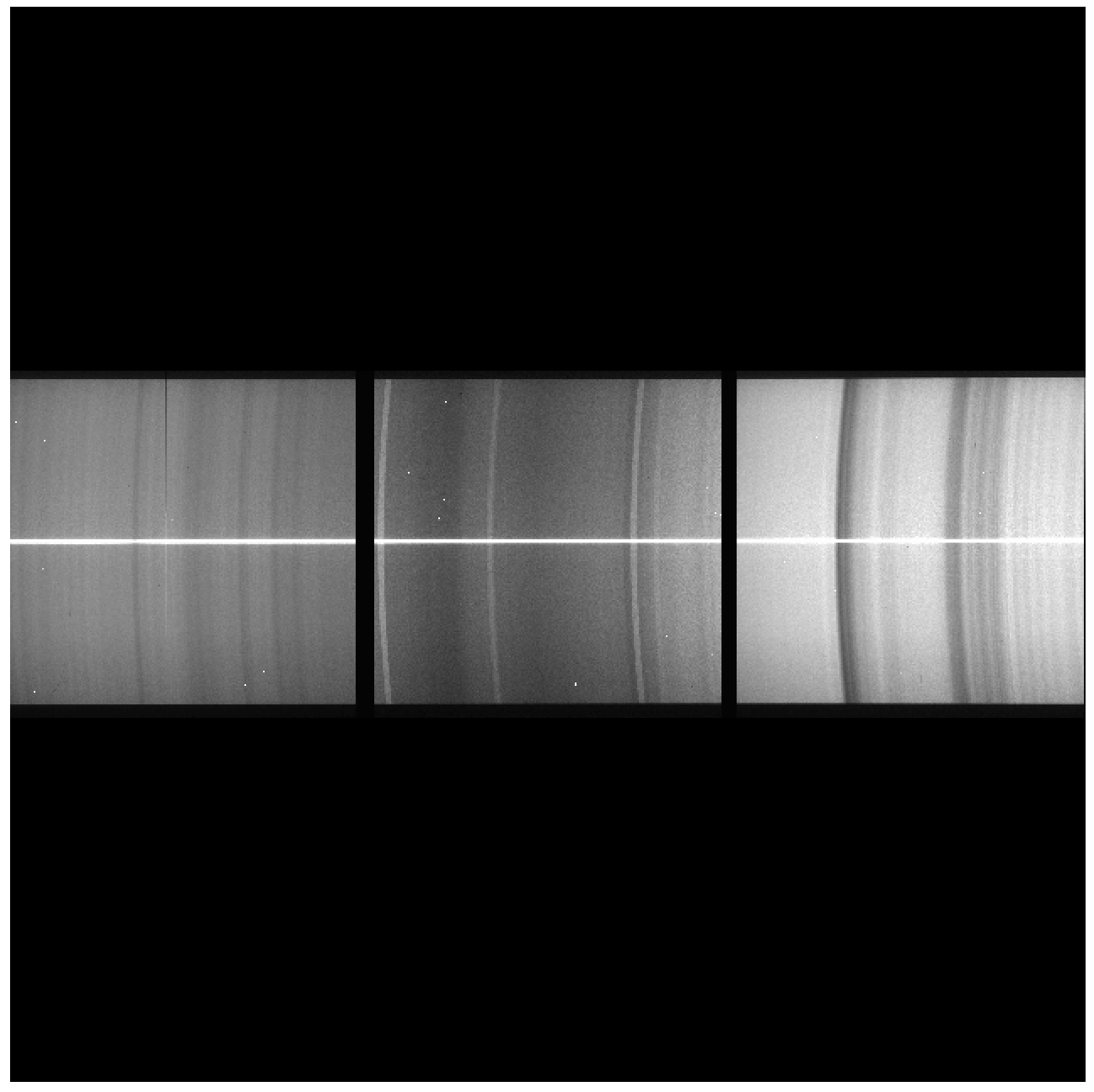
Now, let's take a look at the resulting images:


Notice that the sky lines are straight up and down now, indicating that the wavelength solution has been properly applied.
Background Subtraction
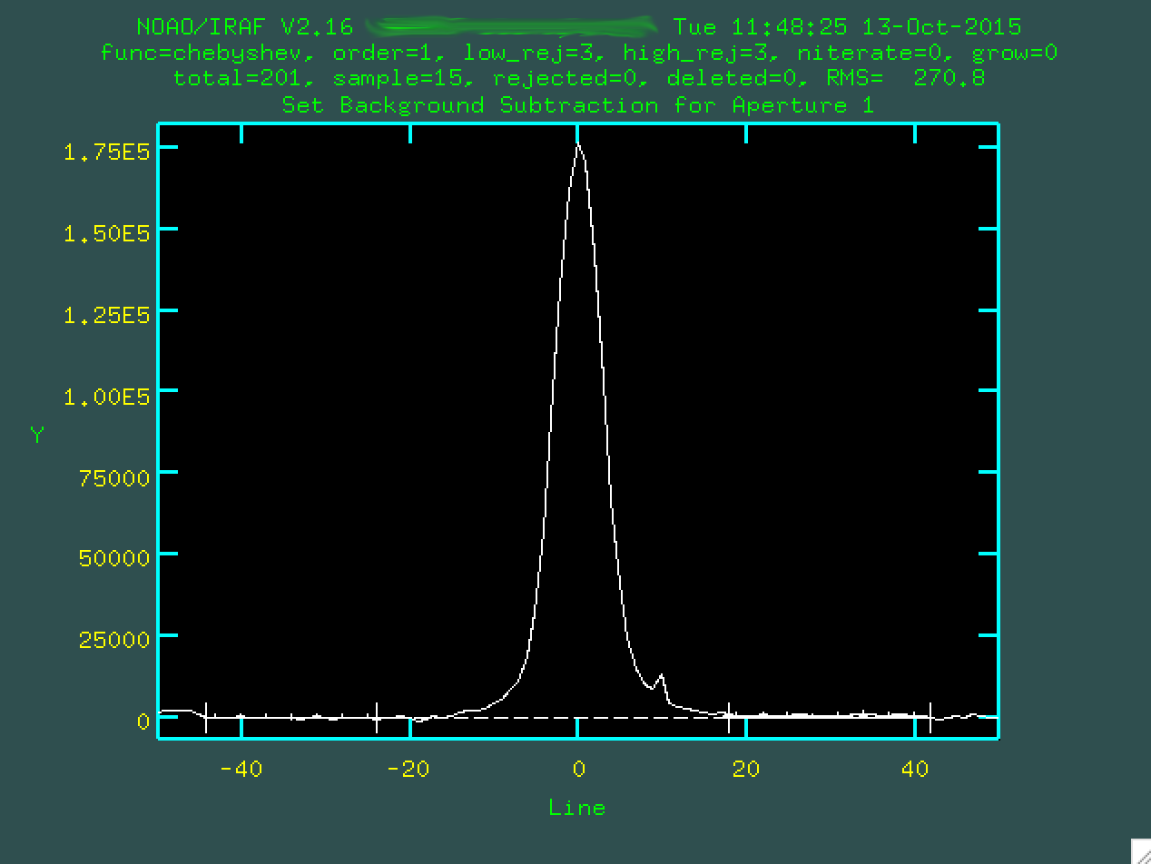
Our next step is to remove the sky lines and any residual sky background flux. This is a process that we want to do on a small region around the central continuum trace of our target, so we could potentially do more trimming, similar to what we did earlier. With this sample data, I think we'll be fine with our original trim region, so let's forge ahead.
For running our background subtraction, we'll use the appropriately named
IRAF task background:
  > background input=J135925.sci.32.t.trim.fits output=J135925.sci.32.tb.trim.fits axis=2 interactive=yes naverage=1 function=chebyshev order=2 low_rej=2 high_rej=1.5 niterate=5 grow=0
  > background input=J135925.sci.33.t.trim.fits output=J135925.sci.33.tb.trim.fits axis=2 interactive=yes naverage=1 function=chebyshev order=2 low_rej=2 high_rej=1.5 niterate=5 grow=0
  > background input=J135925.sci.34.t.trim.fits output=J135925.sci.34.tb.trim.fits axis=2 interactive=yes naverage=1 function=chebyshev order=2 low_rej=2 high_rej=1.5 niterate=5 grow=0
When you run this, you'll find that an irafterm window will open up, like
when we ran identify or fitcoords. This one is a little
easy to miss, though:

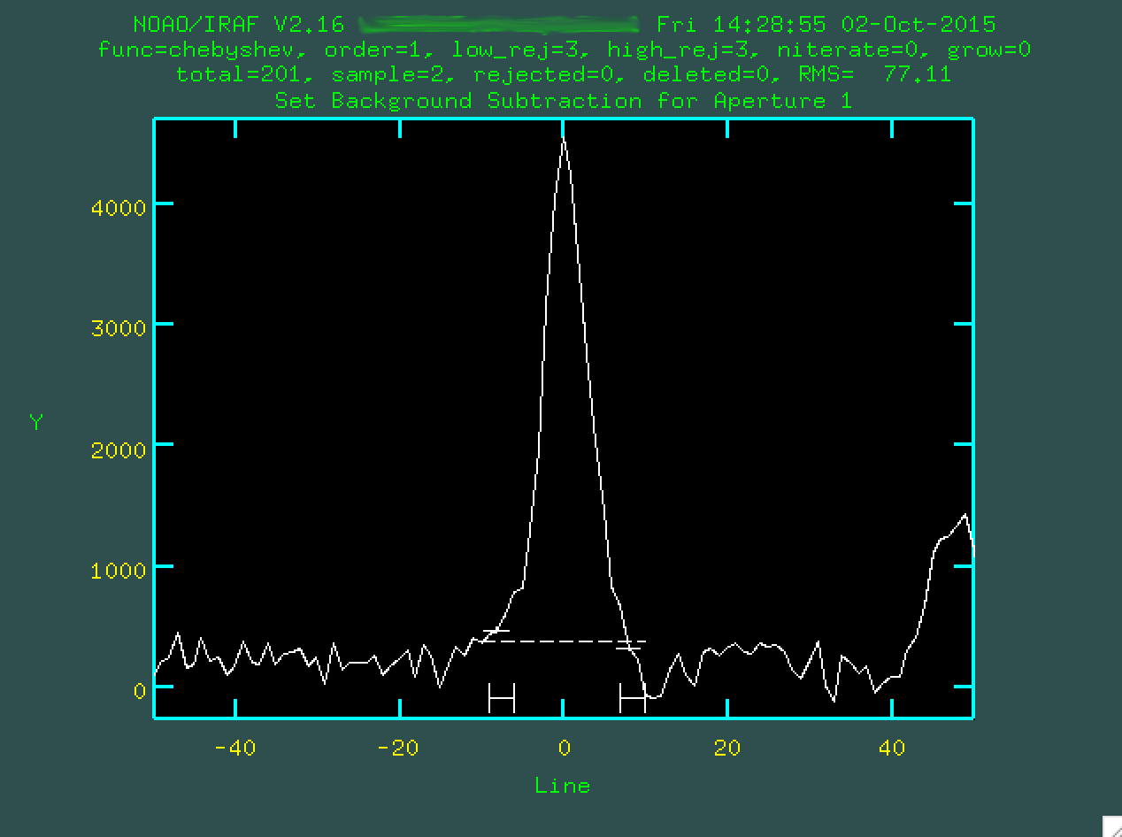
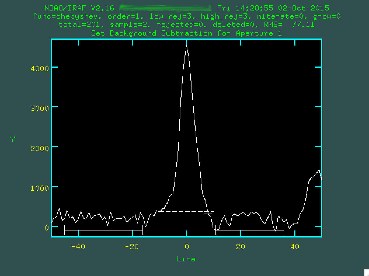
This window is patiently waiting for you to provide a set of columns with
which to measure the sky background value with respect to the central trace. I
tend to use a region that actually shows some bright central trace emission for
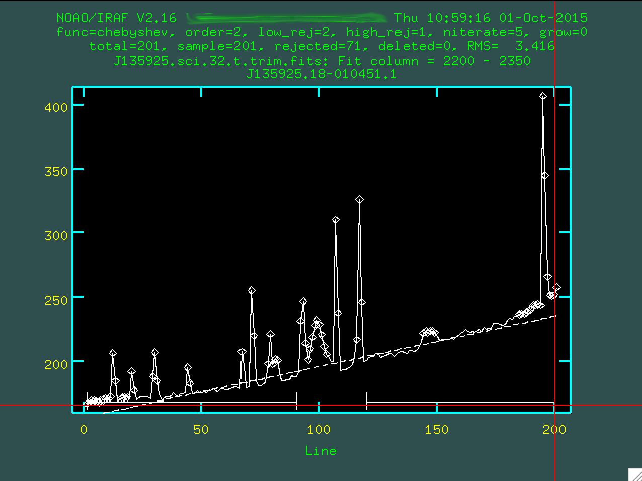
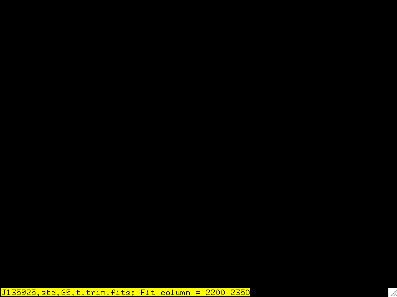
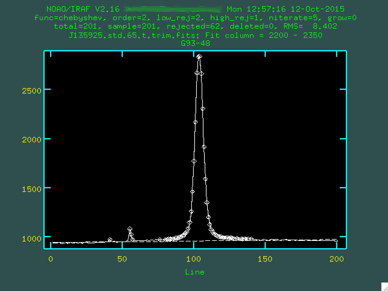
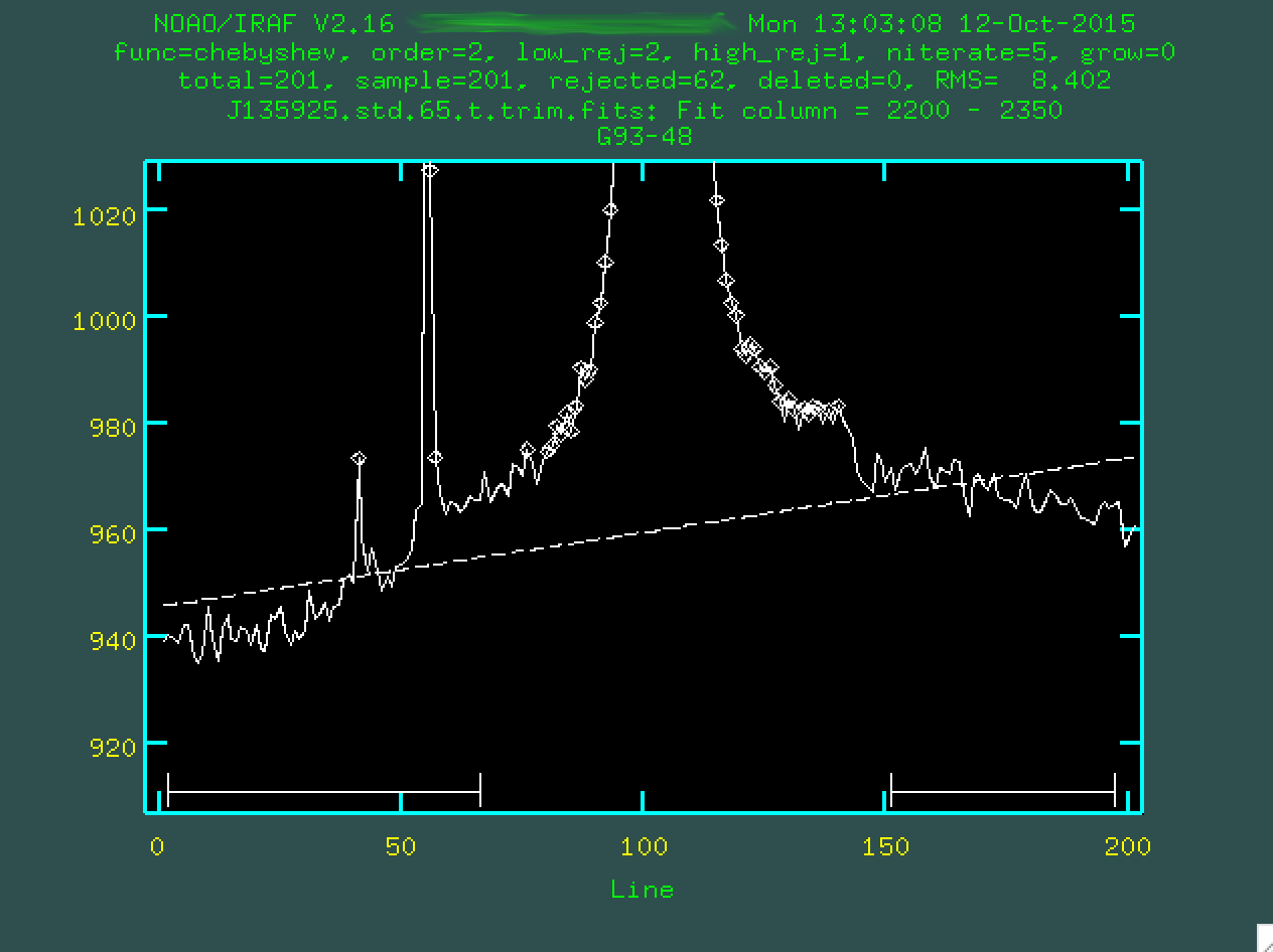
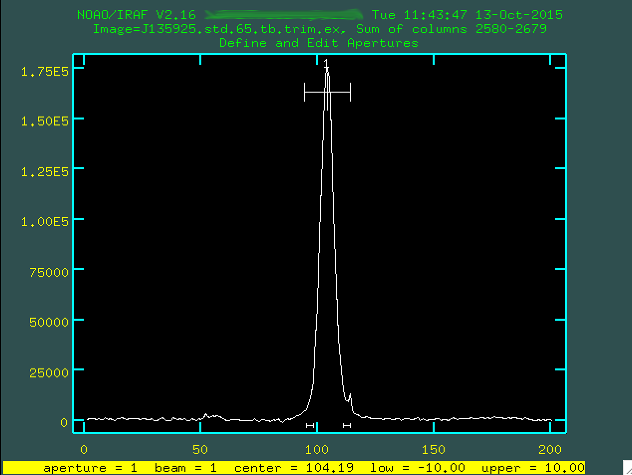
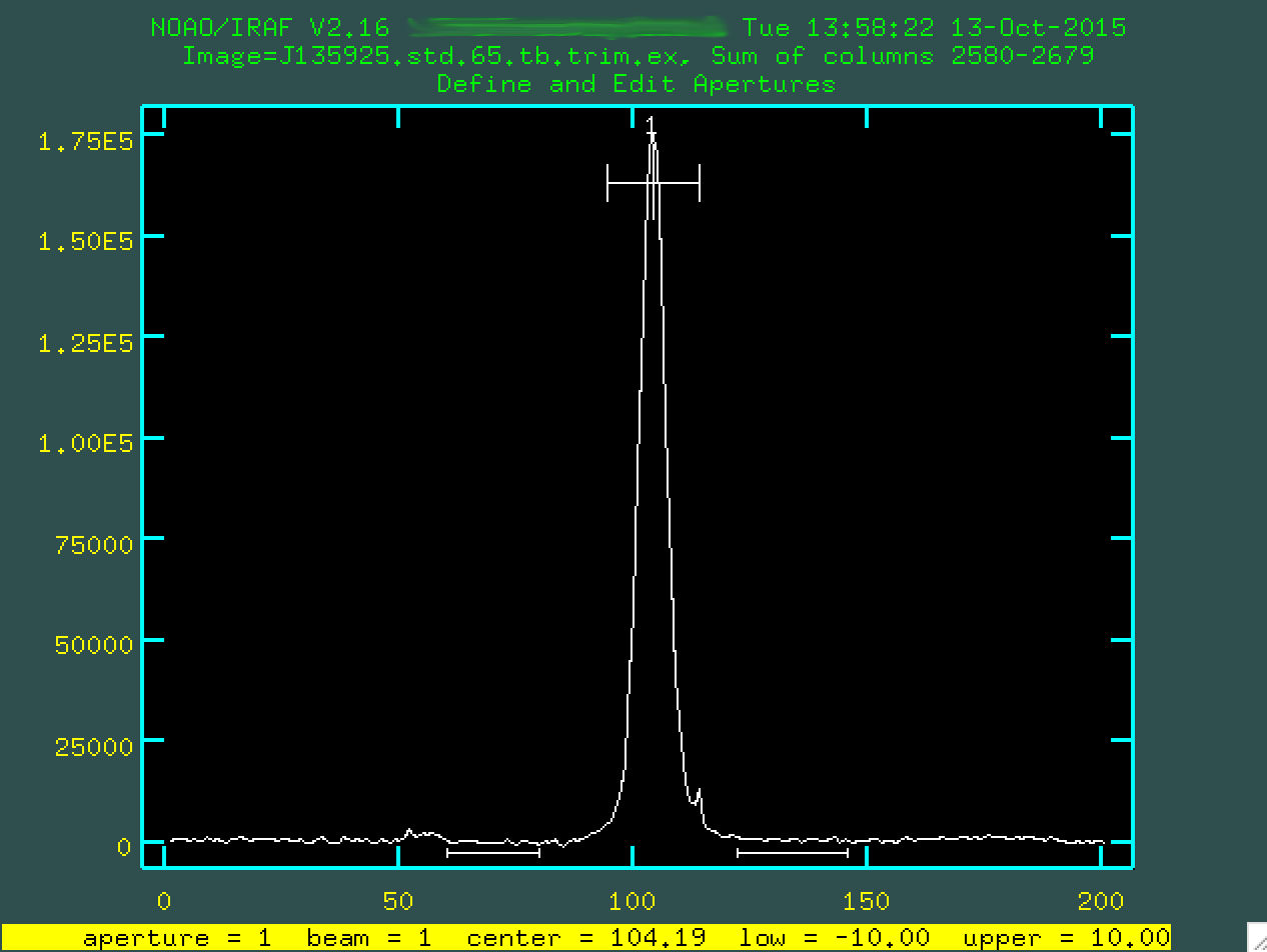
this purpose, like in the region in our images at around 2200 - 2350. Make sure to
not to include any sky lines in this region! So, here, I'll type 2200 2350...

...and press enter.
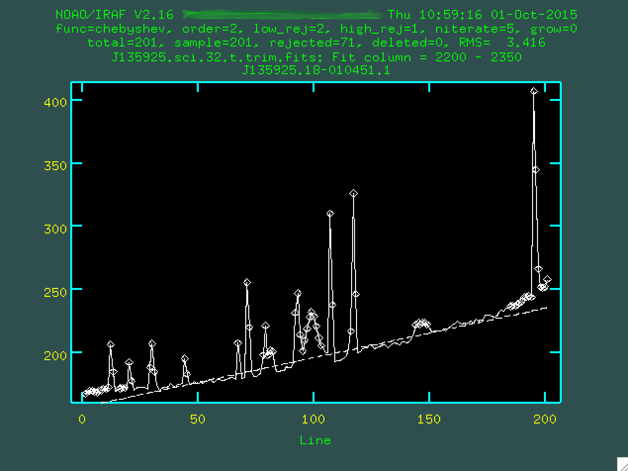
Now, what you're seeing here is what happens when you take the 2D spectrum and compress it in the wavelength direction, but only for the region between columns 2200 - 2350. The curve upward to the right is the gradual increase in brightness, probably due to light from that bright star just above our target. The big spikes are the result of cosmic rays hitting our detector while we were exposing the data. And, right there in the middle, the tiny hump at 100, that's our trace. It's faint, but it's there.
There's also a straight dashed line, which represents the initial fit, which
we specified as being second order by setting order=2 when we called
background. It does an ok job, but we can do better. But first, we
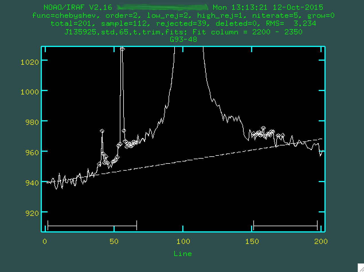
should specify the region that we want to use to measure the background. To do
this, you have to type s at the leftmost part of a region that
contains the background, and then s at a point to the right of
where the background is. So, for instance, I clicked s here:
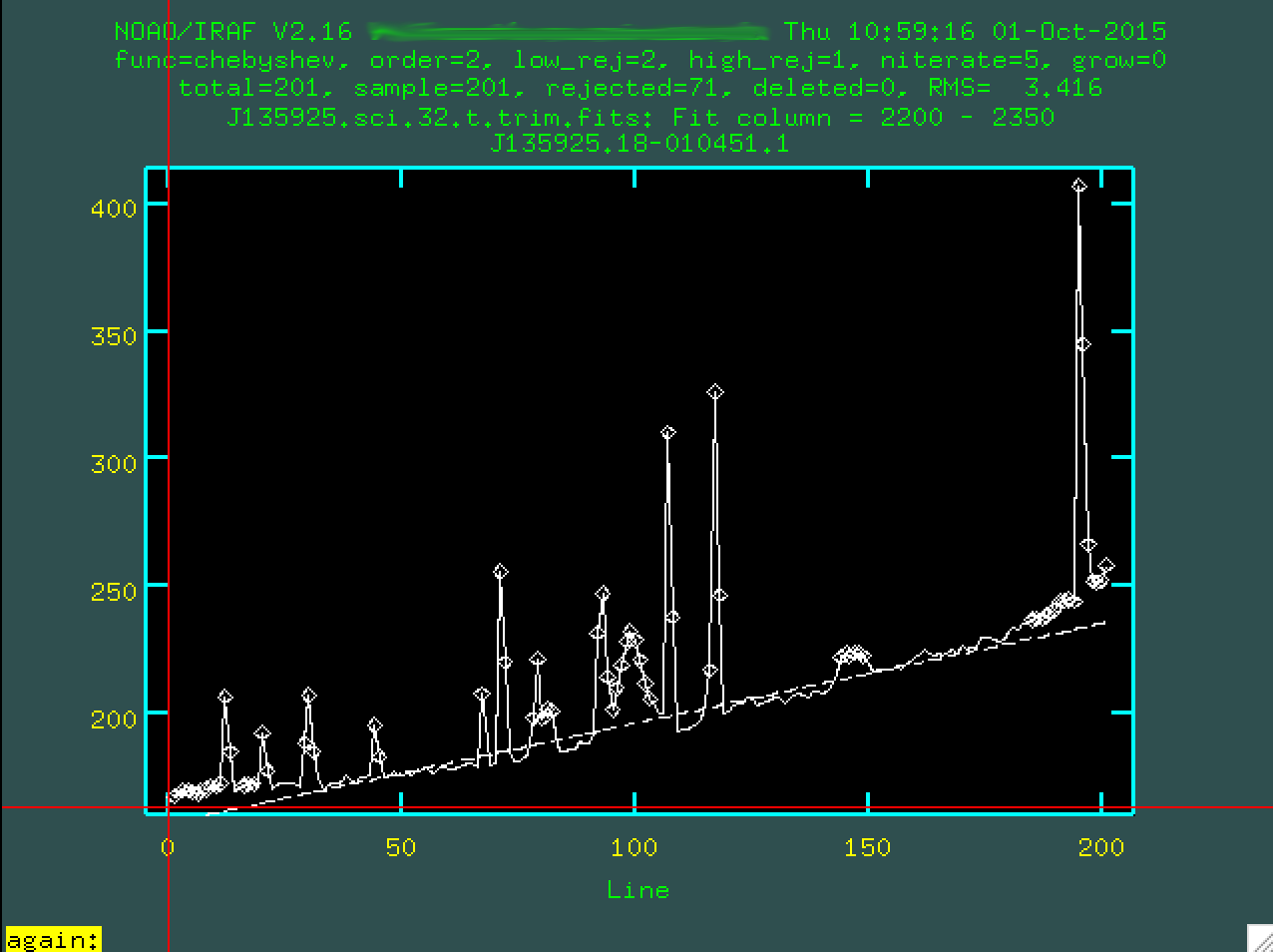
And then again here:
I'll do the same on the other side of the central trace, too.
You want to define the background with regions that are right up to the edge
of the actual trace, so it doesn't try to use the trace to constrain the
background subtraction. You can then change the order by typing :or 3
(or 4, or 5 or whatever you think fits best, I'm going to go with 3), then you re-fit
by typing f:
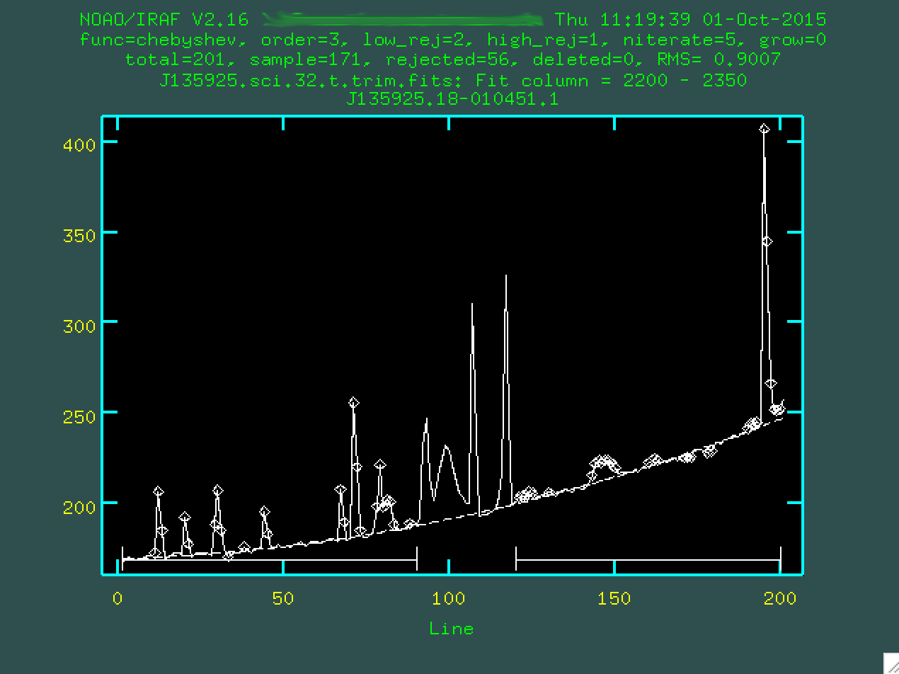
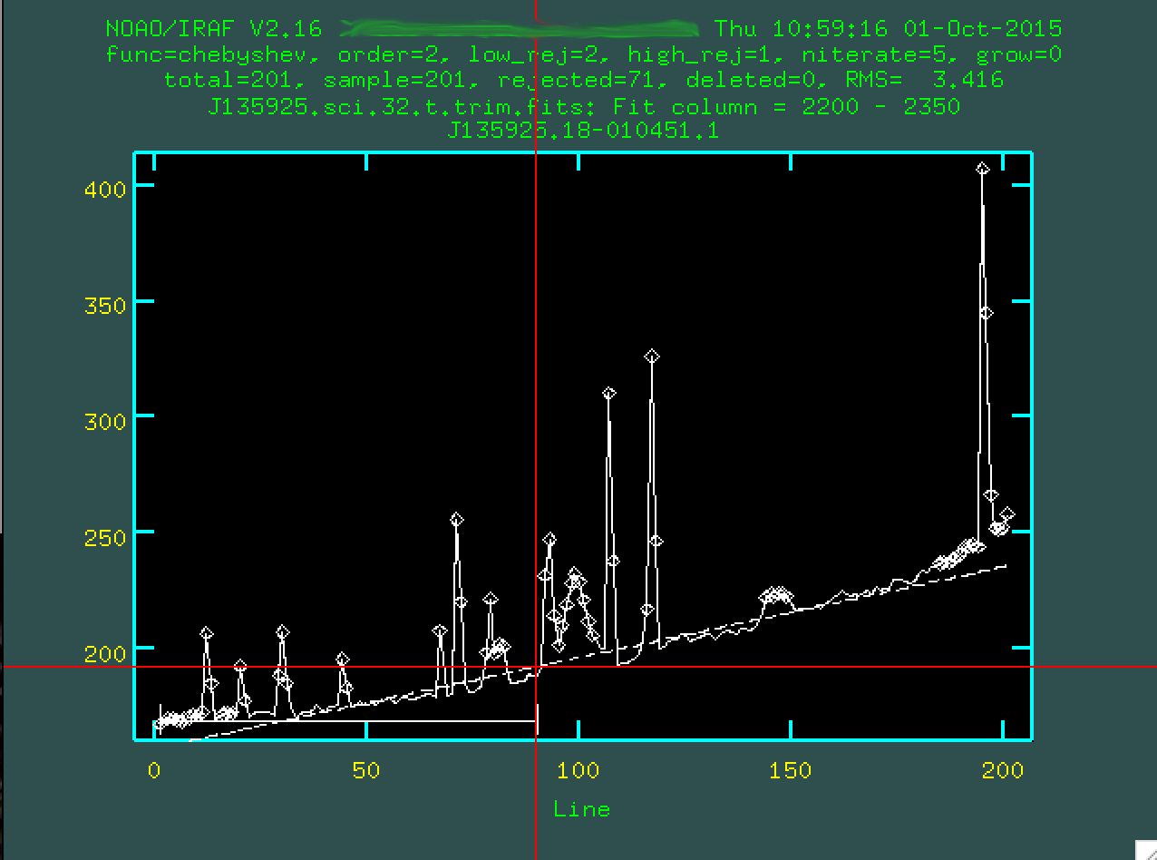
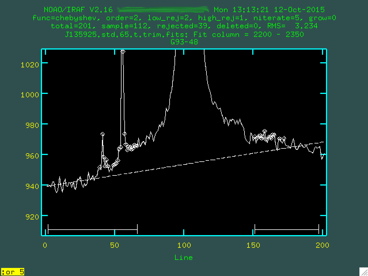
Hopefully, the dashed line goes through the background points. It might help
to zoom in, too, similar to what we did with identify, by typing
w then e on the bottom left corner of the zoomed in
region I want, and then e on the top right corner of the zoomed in
region I want.
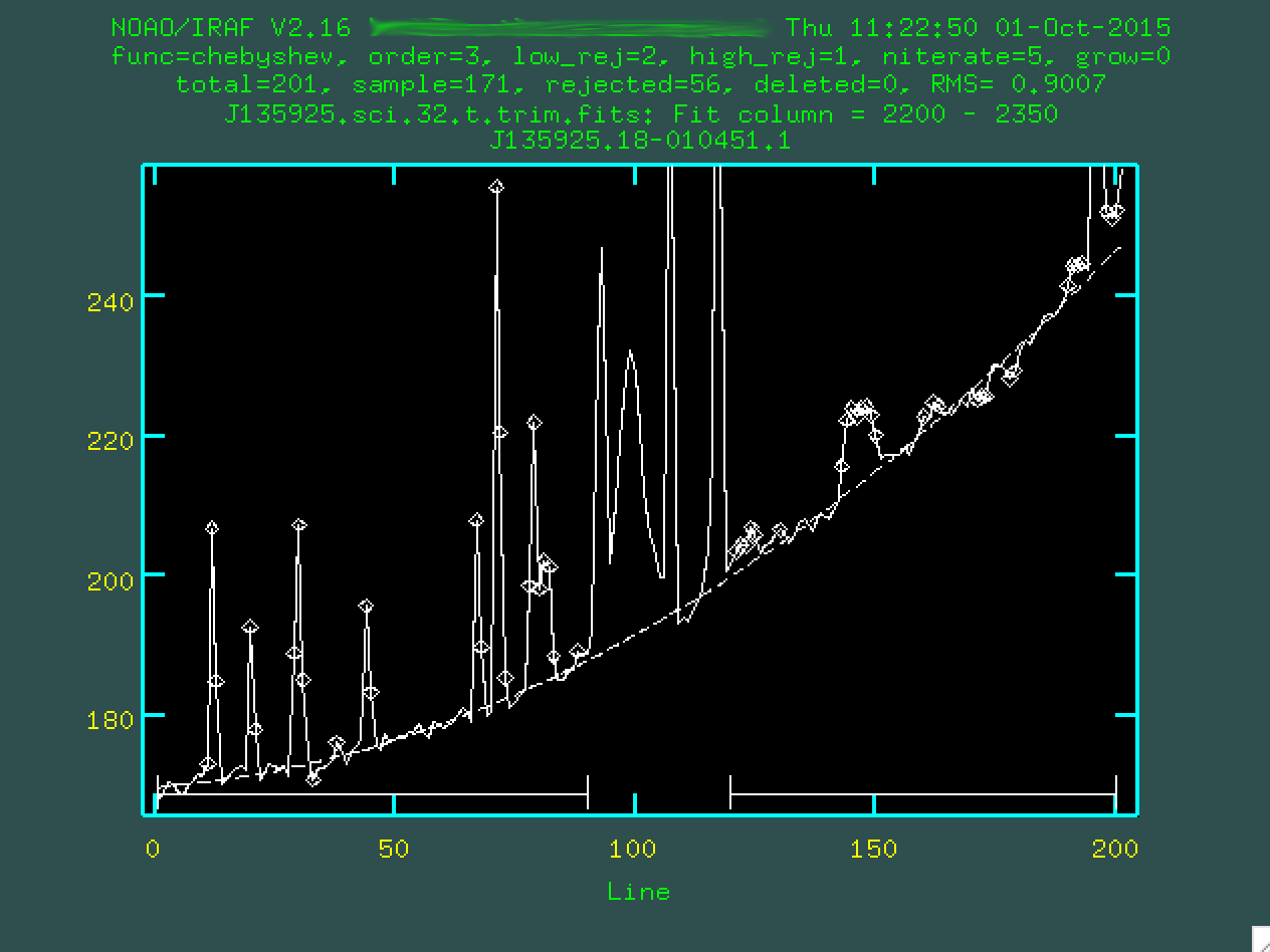
This looks pretty good. So, now you type q, and then press enter.
At this point, the code will chug along for a bit, removing the background
from the entire image using this model. When it's done, take a look at the
resulting image. The sky lines should be gone, and the background level should
be noisy, but zero-ish. You'll still see the cosmic rays, which we'll deal
with in the next step.

If you want to double check your background subtraction, you could use the
IRAF task implot to take a better look at what you just did:
> implot J135925.sci.32.tb.trim.fits
You can just plot a column of interest by typing something like :c 2100 2700,
which will plot columns 2100 to 2700 collapsed, and should look very similar to what
you saw when you were background subtracting, but the background levels have
been subtracted out.
Now, once you've done this for all of the images, let's combine the data.
Imcombine Science Images
Now, before we run imcombine, we have to make sure that everything
is lined up from image to image. This is only an issue if your object has
moved with respect to the slit, so I would go and open all three of the background
subtracted images and look to see if the trace moves up or down in any of the
images. There is a description for how
to do this process in a rigorous manner here (scroll down a little), in
case you want to do this. For this SALT example, I don't know if it's necessary,
since the object doesn't look as if it slid very far.
Either way, we are going to use imcombine, along with our bad pixel
masks, to create a combined science image, as well as an error image. Before
we combine the images, we have to make sure that the image header has the
trimmed bad pixel mask. When imcombine takes the three science
exposure and combines them, it will use the bad pixel masks given using the BPM header
keyword. So, first, let's take a look at the header, using imhead:
> imhead J135925.sci.32.tb.trim.fits l+
Here, l+ tells IRAF that you want the whole header. Scroll down (in IRAF,
scrolling is accomplished through a "middle click", which you can do on a Mac
by holding down option while you click on the scroll bar.) and look for the
header keyword BPM:
BPM = 'crmask_J135925.sci.32.trim.pl'
Now, we want this to actually have crmask_J135925.sci.32.t.trim.pl, instead,
so we can use the IRAF task ccdhedit, found in noao.imred.ccdred:
> ccdhedit crmask_J135925.sci.32.trim.pl BPM "crmask_J135925.sci.32.t.trim.pl"
Now, if you check the image header (same as above, use imhead and
l+, and you'll hopefully see that the BPM header now
reads crmask_j0911.1076.bft.trim2.pl. The second way that you can
edit the image header is using the IRAF task eheader, found in
stsdas.toolbox.headers:
> eheader crmask_J135925.sci.32.trim.pl
This is going to open up the whole image header for you to edit. By default,
the editor that IRAF uses is vim, which is a pretty crazy text editor. If you
want to edit anything, move the cursor down to where you want to make the edit
using the up/down/left/right arrows on the keyboard, then press i to
go into "insert mode," and now you can add in the text you want (like the 2 in our
example above), and then you press esc to escape out of insert mode,
and then finally :wq to save and quit the image header editing. It's
a bit of a process.
Anyway, now it's time to run imcombine. First, we want to create
a list of the files we are going to combine:
ls *tb* > J135925.list
And now we have a file called "J135925.list" which has three entries, the
names of the three files. Now we can go and run imcombine:
> imcombine @J135925.list J135925.med.fits sigma=J135925.med.sig.fits combine=median scale=mean statsec=[2164:2297,130:180] masktype=goodvalue
Some text will be written to the screen:
  Oct  1 15:17: IMCOMBINE
    combine = median, scale = mean, zero = none, weight = none
    blank = 0.
    statsec = Oct  1 15:17
    masktype = goodval, maskval = 0
                  Images     Mean  Scale Maskfile
    J135925.sci.32.tb.trim.fits  2.5812  1.000 crmask_j135925.sci.32.t.trim.pl
    J135925.sci.33.tb.trim.fits  2.9755  0.867 crmask_j135925.sci.33.t.trim.pl
    J135925.sci.34.tb.trim.fits  4.0669  0.635 crmask_j135925.sci.34.t.trim.pl

    Output image = J135925.med.fits, ncombine = 3
    Sigma image = J135925.med.sig.fits
And you should see which images were stacked, and which cosmic ray masks were used. The output will be two files, J135925.med.fits and and J135925.med.sig.fits, since we used a median combine on the images. We've also scaled them by their means, which is why you see the scale values listed in the output text.
So, let's go and take a look at the final image:

You can see our strong trace running through the center, and some strong emission lines along the trace. If you are familiar with the strong optical emission lines present in a star-forming or active galaxy, you should be excited. ALSO, can you see the other thing that is exciting about these reduced data? Just above the trace is another trace, with emission lines at the same redshift, indicating that we got lucky with our slit placement and managed to also cover a galaxy that might be in a merger with J135925. Really exciting! Let's now run a few corrections and extract the primary aperture.
Make The Variance Image
This is a straightforward step. We're going to take the recently created sigma image, and turn it into a variance image. We'll use this to extract error variance spectra, which we can turn into sigma spectra:
  > imcalc J135925.med.sig.fits J135925.med.sig.sqr.fits "im1**2"
  > imcalc J135925.med.sig.sqr.fits J135925.med.var.fits "im1/3"
  > imdel J135925.med.sig.sqr.fits
So, here, we are first taking the square of the sigma image, and then dividing by the number of images that went into making it, which creates the variance image. Finally, we delete the squared image. In a future step, when we extract a spectrum from the variance image, we're going to want to take the square root of it to get the sigma spectrum, which is our true uncertainty on the spectral values.
Extinction Correction
So, before we extract, we can run extinction correction based on the airmass.
To do this, however, we have to put some information in the headers. The headers
for these image we've been working with are a little sparse, thanks to our using
imcopy to pull out the images to work with in IRAF earlier. We
need the AIRMASS, EXPTIME, and st header parameters, which we can get from
the original product images:
> imhead mbxgpP201505180032.fits[0] l+
And then find these three keywords:
  EXPTIME =              800.199 / Exposure time
  AIRMASS =       1.282297036574 / Air mass
  TIME-OBS= '19:00:37.535'       / UTC start of observation
And now, update the header for both the .med. and the .med.var. files to include these header keywords.
   > hedit J135925.med.fits EXPTIME 800.199
   > hedit J135925.med.fits AIRMASS 1.282297036574
   > hedit J135925.med.fits st "19:00:37.535"
WARNING: hedit is a powerful program used to update image
header keywords, and you can totally overwrite existing keywords, which
is non-ideal. Make sure you take a look at the parameters for hedit:
  PACKAGE = imutil
     TASK = hedit

  images  =     J135925.med.fits  images to be edited
  fields  =                   st  fields to be edited
  value   =         19:00:37.535  value expression
  (add    =                   no) add rather than edit fields
  (addonly=                  yes) add only if field does not exist
  (delete =                   no) delete rather than edit fields
  (verify =                  yes) verify each edit operation
  (show   =                  yes) print record of each edit operation
  (update =                  yes) enable updating of the image header
  (mode   =                   ql)
These settings will allow you to update the header, but will ask you before making changes. Do the same thing for the variance image:
   > hedit J135925.med.var.fits EXPTIME 800.199
   > hedit J135925.med.var.fits AIRMASS 1.282297036574
   > hedit J135925.med.var.fits st "19:00:37.535"
Now, with this done, we'll use the extinction program, which is part of the
noao.twodspec.longslit package:
  PACKAGE = longslit
       TASK = extinction

    input   =   J135925.med.fits  Images to be extinction corrected
    output  = J135925.med.ex.fits  Extinction corrected images
    (extinct= onedstds$ctioextinct.dat) Extinction file
    (mode   =                   ql)
So, you can see here that we've set extinct=onedstds$ctioextinct.dat which is
the CTIO standard extinction file, ideal for southern hemisphere targets. You run
the program in this way:
   > extinction J135925.med.fits J135925.med.ex.fits
    Extinction correction: J135925.med.fits -> J135925.med.ex.fits.
This will run using the Zenith Distance (given as ZD in the header), in a way described here. Make sure to run this same process on the variance image, as well:
   > extinction J135925.med.var.fits J135925.med.var.ex.fits
    Extinction correction: J135925.med.var.fits -> J135925.med.var.ex.fits.
Primary Aperture Extraction
Now that we have our stacked 2D spectrum, we want to extract a 1D spectrum.
For aperture extraction, we'll be using the IRAF program apall, which
is part of the noao.twodspec.apextract package. I have put a .cl
script here, which we'll use to extract our 1D
spectrum.
We're going to modify this script, and then run it, which will call
apall. Apall will look for a peak in some column range
that we give it (the first part will look a lot like our implot runs
above). Then, armed with this position of the central trace in the spatial
(up and down) direction, it will trace the whole spectrum in the wavelength
direction.
So, open up apall.sci.cl in your favorite editor. First, we're
going to want to change apall.input to the name of the reduced fits
file we just created, and change the output to be whatever we want.
    apall.input="J135925.med.ex.fits"
    apall.nfind=1
    apall.output="J135925.med.ex.ms"
    apall.apertures=""
    apall.format="multispec"
    apall.references=""
    apall.profiles=""
Next we'll want to make sure that a series of flags are set correctly for what we want to do on the first pass. We want to do this interactively, and we want the program to find the central aperture. We don't need to recenter, or resize, but we'd like to edit the apertures (so we can look at them). We want to trace the aperture in the velocity direction, and fit to that trace, and finally, we want to extract the aperture.
    apall.interactive=yes
    apall.find=yes
    apall.recenter=no
    apall.resize=no
    apall.edit=yes
    apall.trace=yes
    apall.fittrace=yes
    apall.extract=yes
    apall.extras=no
    apall.review=no
Now, these next lines are important. apall.line should be set to the
central row/column pixel value of the range you care about, in pixel units. If
you have a faint object, this might just be some bright emission line. Here,
we have a medium-bright continuum, let's use a range near the [OIII] emission
lines. The value for apall.nsum is how many lines/columns you want to sum
around that central pixel value. Finally apall.lower and
apall.upper are the spatial size (in pixels) of the aperture on
both sides of the center. Generally you'll set these both to the same size.
So. If you want a twenty pixel wide aperture, and you want to look from 2580 - 2680 (which is to the red of [OIII] 5007), you'd set things this way:
    apall.line=2630
    apall.nsum=100
    apall.lower=-10
    apall.upper=10
Leave the rest as it is, as it's stuff relating to the trace, and weights,
but change the final line, so that apall is actually called:
apall J135925.med.ex.fits
So, now, we can run the script:
> cl < apall.sci.cl
The script will run, and you will be asked a series of questions:
  Find apertures for J135925.med.ex?  (yes):
  Number of apertures to be found automatically (1):
  Edit apertures for J135925.med.ex?  (yes):
You set all of this in the script, so you can probably press "enter" to go through this all. You'll eventually get to the a screen showing a 2D slice in the region you specified:

In the center, we can see the trace. To the right of that, the peak you
are seeing is the other object along the slit. Now, we have specified, in
the running of apall that apall.background="none",
which meant that we didn't want to do further background subtraction. If we had,
instead, wanted to do more background subtraction, we'd want to define the
background outside of the trace. To do that, we'd type b, and we'll be
presented with this screen:
Here, like many of these screens, we could zoom in with w and
e. With this example, it's zoomed in pretty well, so we can now
just delete the original background regions by hovering over them with the mouse
and typing z. At this point we can define our own background
regions exactly like what was done using background earlier, by typing
s on either side of the regions you want to use. Here are my
final regions for defining the background:
I'm happy with these regions, so type f to refit the background:
And now I can type q to get back to the original screen, with
the new background defined.
As a side note, sometimes you may find that the program has automatically selected a different trace than you had wanted to. Or, in this case, perhaps you want to select the secondary object instead of the central trace.
If this is the case, you are going to want to delete your original trace
by hovering over the point and the range above the trace (labelled with 1) and
typing d. At this point you can hover over another trace region
you want and then type m. You can redefine the width of the
aperture by moving your mouse to the side of the trace and then typing y,
which sets the width to that size.
Once you're happy with the central trace, and the background, again, type
q. The program will then ask if you want to trace the apertures,
so type yes or press enter if yes is already selected. You will be
asked if you want to fit the traced positions interactively, and we want to, so
type yes, or just press enter if yes is already given. You'll then
be asked if you want to fit a curve to aperture 1, and again, type yes or press
enter if yes is already selected.
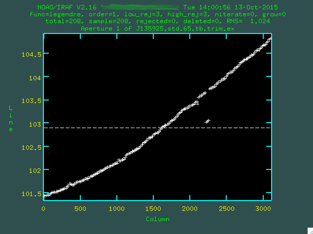
At this point you'll be presented with another screen, which shows the intial fit to the trace along the wavelength direction.
Here, you can see what happens when apall tries to find the
trace outside of the range you defined above. It's a little noisy, but you can see
that it's definitely slanted with respect to the image. The horizontal line is
our first order fit, which obviously doesn't fit very well. We can fit a higher
order fit, like a 4th order polynomial, by typing :or 4, and pressing
enter. Choose whatever order fit you think works the best, but don't go
too high, since you'll start just overfitting the data.
Now, you can update your fit by typing f, which will refit things.

If you want to delete outlier points, you can hover over them and type d,
and make sure to refit using f. Here's the final fit that I used:
Now, if you type q, you'll quit out of this process, and
when asked if you want to write the apertures to the database, type yes
(or press enter if yes is already selected), and then when asked if you want
to extract the aperture, type yes (or press enter if yes is already selected).
This whill save the fit to a 1D spectrum file, which in this case is known
as "J135925.med.ex.ms.fits", as per what we specified in the apall
script. You can look at the fit with splot:
> splot J135925.med.ex.ms.fits
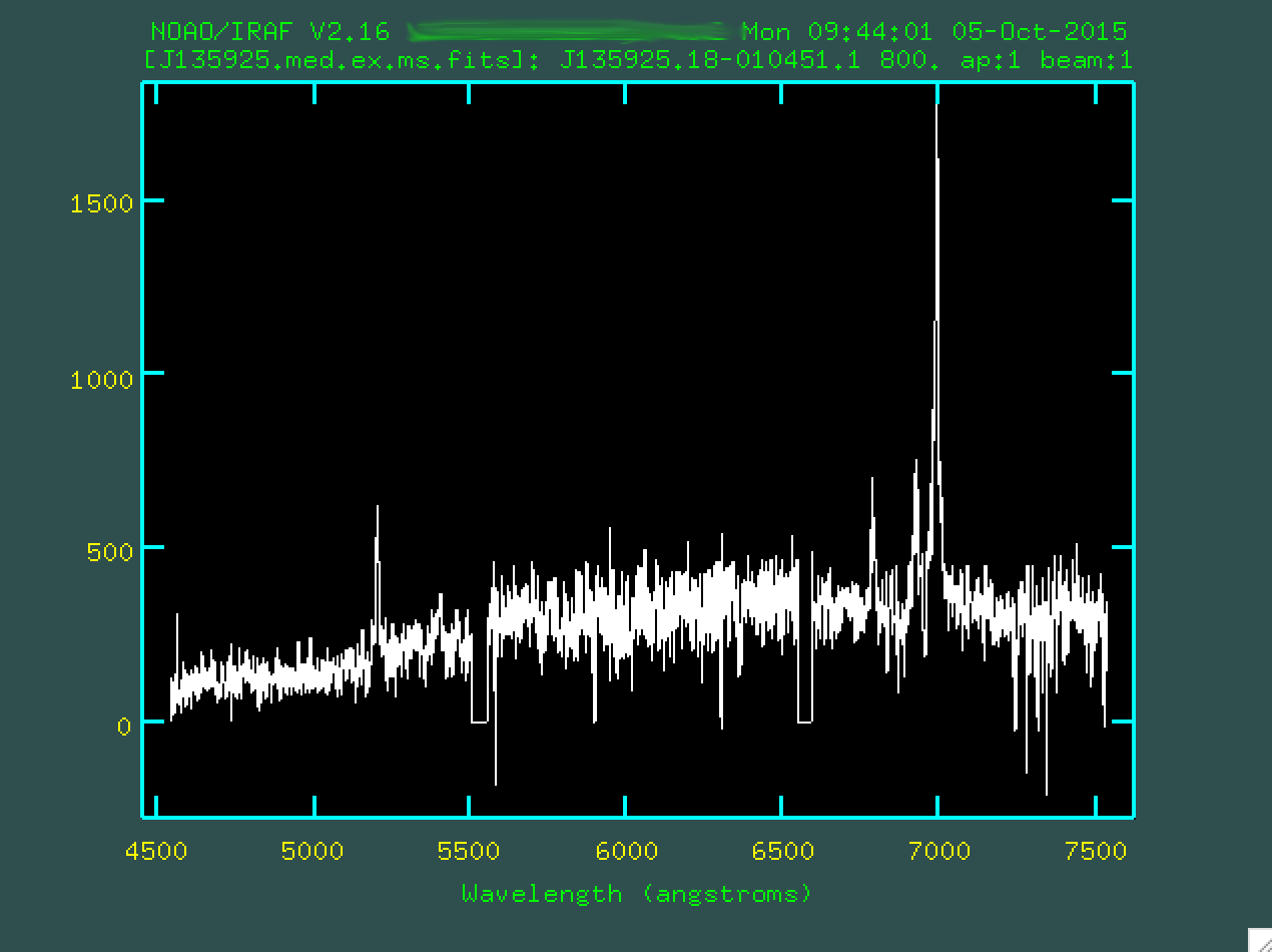
This looks great! You can see all of our strong emission lines. You can go and redo this to your hearts content if you're not happy with how that worked. The program has created a file in the folder "database", which in the case of the example is called "J135925.med.ex". If you do want to redo the full extraction and tracing, delete this file first, so that the version you edit only has a record of one extraction, the last one that you did.
Now, we're going to want to go and extract an error spectrum. It's pretty straightforward. What you want to do first is copy over your apall.sci.cl script to another version that we'll call apall.sci.err.cl, for lack of a better name. We'll need to change a few things here:
   apall.input="J135925.med.var.ex"
   apall.nfind=1
   apall.output="J135925.med.var.ex.ms"
   apall.apertures=""
   apall.format="multispec"
   apall.references="J135925.med.ex"
   apall.profiles=""

   apall.interactive=no
   apall.find=no
   apall.recenter=no
   apall.resize=no
   apall.edit=no
   apall.trace=no
   apall.fittrace=no
   apall.extract=yes
   apall.extras=no
   apall.review=no
   ...
   apall J135925.med.var.ex.fits
Notice a few things. First, you are using a reference trace, which in this case is the trace you just extracted on the actual data. Also, you want to run this is noninteractive mode, you don't want to find, recenter, resize, edit, or fit to the trace. You do want to extract the spectrum, though! This will run the same exact aperture extraction as you just did, except on the variance image. So, run it:
> cl < apall.sci.err.cl
Once you extract a variance spectrum, you're going to want to turn this into a sigma spectrum to find the error at each wavelength:
> sarith J135925.med.var.ex.ms.fits sqrt "" J135925.med.sig.ex.ms.fits
Which takes the square root of the variance image and produces the sigma image, the error spectrum.
Flux Calibration
So, our next step is to reduce the standard star spectrum in order to run the relative flux calibration. You can run the reduction of the standard star spectrum in the same folder that you're running your object reduction, but also, it's possible to run everything in a different folder, providing you copy over the trimmed arc image and the database folder (with the files inside) to where you run the standard star reduction. It is never a bad idea to separate out your reduction steps into various folders so that if you make a mistake, or want to redo a step, it's more straightforward to find the file that need to be changed.
The standard star file is mbxgpP201505220065.fits. Now, standard star spectra, at least with SALT, are a little bit of a tricky thing. You should have standard star spectra for your project, providing you've requested these observations. They may not be taken in the same night as your observations, but you can use spectra for a different night (one as close to the same night as you can) providing the instrument is set up the same way. You don't want to apply an incorrect wavelength transformation to a standard star spectrum. You can look up the instrument configurations for the science and standard images in their headers:
   > imhead mbxgpP201505180032.fits[0] l+
   ...
  PROPID  = '2015-1-SCI-052    ' / Proposal ID
  OBJECT  = 'J135925.18-010451.1' / Target Object
   ...
  GR-ANGLE=            15.875000 / Grating Rotation Angle (encoder)
  GRATING = 'PG0900            ' / Commanded grating station
  FI-STA  = '5                 ' / Commanded Filter Station
  FILTER  = 'PC03850           ' / Filter Bar Code
  CAMANG  =                31.75 / Commanded Articulation Station
vs:
   > imhead mbxgpP201505220065.fits[0] l+
   ...
  PROPID  = 'CAL_SPST          ' / Proposal ID
  OBJECT  = 'G93-48            ' / Target Object
   ...
  GR-ANGLE=            15.875000 / Grating Rotation Angle (encoder)
  GRATING = 'PG0900            ' / Commanded grating station
  FI-STA  = '5                 ' / Commanded Filter Station
  FILTER  = 'PC03850           ' / Filter Bar Code
  CAMANG  =                31.75 / Commanded Articulation Station
Also, notice that the object we're looking at here is the star G93-48, and that website will come in handy when we run the flux calibration.
So, let's get going. Like the other science spectra, we'll want to get this into a format we can work with in IRAF:
imcopy raw_data/mbxgpP201505220065.fits[sci,1] J135925.std.65.fits
From here, we'll want to trim the file. First, let's look at it:
Notice the bright trace across the center of the image. It's going
to fit in well with our original trim, so we could use that. If, however,
we had originally trimmed our science image such that the standard star
spectrum was going to be cut out, we'd have to go and re-trim the arc image,
and then run identify, reidentify and fitcoords
on this new image. This is non-ideal, so be careful when you first trim your
data that you trim a region that will have both the science and the standard
star spectrum in the region.
imcopy J135925.std.65.fits[50:3160,420:620] J135925.std.65.trim.fits
And, as with all of our images, let's take a look:

Now, our first goal is to transform the image, which we can do using the
IRAF task transform. If we're running the standard star reduction
in the same folder as the arc spectrum and the database folder, we can just
run things like this:
> transform input=J135925.std.65.trim.fits output=J135925.std.65.t.trim.fits fitnames=J135925.arc.35.trim interptype=linear flux=yes blank=INDEF x1=INDEF x2=INDEF dx=INDEF y1=INDEF y2=INDEF dy=INDEF
(If you're running the reduction in a separate folder, as I mentioned above, just copy over J135925.arc.35.trim.fits and the database folder to your working directory before running that line.
When you run transform, you'll get some output:
  NOAO/IRAF V2.16 XXX@XXX Mon 12:31:41 12-Oct-2015
    Transform J135925.std.65.trim.fits to J135925.std.65.t.trim.fits.
    Conserve flux per pixel.
    User coordinate transformations:
      J135925.arc.35.trim
    Interpolation is linear.
    Using edge extension for out of bounds pixel values.
    Output coordinate parameters are:
      x1 =      4542., x2 =      7535., dx =     0.9624, nx = 3111, xlog = no
      y1 =         1., y2 =       201., dy =         1., ny =  201, ylog = no
  Dispersion axis (1=along lines, 2=along columns, 3=along z) (1:3) (1):
You can press enter to finish the fit, and you'll notice
a new file has been created, J135925.std.65.t.trim.fits:

This looks pretty good. So, now we want to run the background subtraction on this image. We won't need to remove cosmic rays, since there aren't a huge number of them, as this is a short exposure. You could, I suppose, so it's up to you.
Next, let's run background on the image:
background input=J135925.std.65.t.trim.fits output=J135925.std.65.tb.trim.fits axis=2 interactive=yes naverage=1 function=chebyshev order=2 low_rej=2 high_rej=1.5 niterate=5 grow=0
As we saw with the previous run of background, you'll be
initially presented with a request:
Again, we should use a region that doesn't have chip gaps or sky feautres.
Let's just use the same region we used in the science data, 2200 - 2350. So,
here, we'd type 2200 2350:
And then we'd press enter.
Here, we're seeing a 2D spectrum compressed in the wavelength direction
between the values we specified. The central peak is the center of the trace,
and you can see the fit below with a dashed line. We're going to want to zoom
in, so we can do that using w e and e to specify
the corners, in ways we've done before.
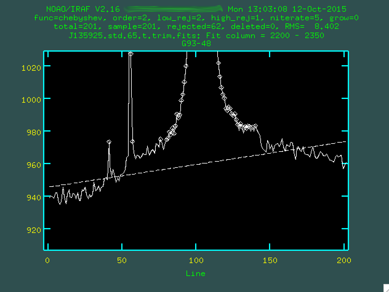
So, in the zoom-in, you notice that the fit doesn't do a great job. Let's
make things better by defining the region on either side of the central trace
where we can measure the background. Again, we'll type s on either
side of the regions we want to define as the background.
And if we type f, it will redo the fit using those regions:
As you can see, the results aren't great, so we should change the order
of the fit. I went with a 5th order polynomial, by typing :or 5
and pressing enter:
And we'll want to type f to refit the background:
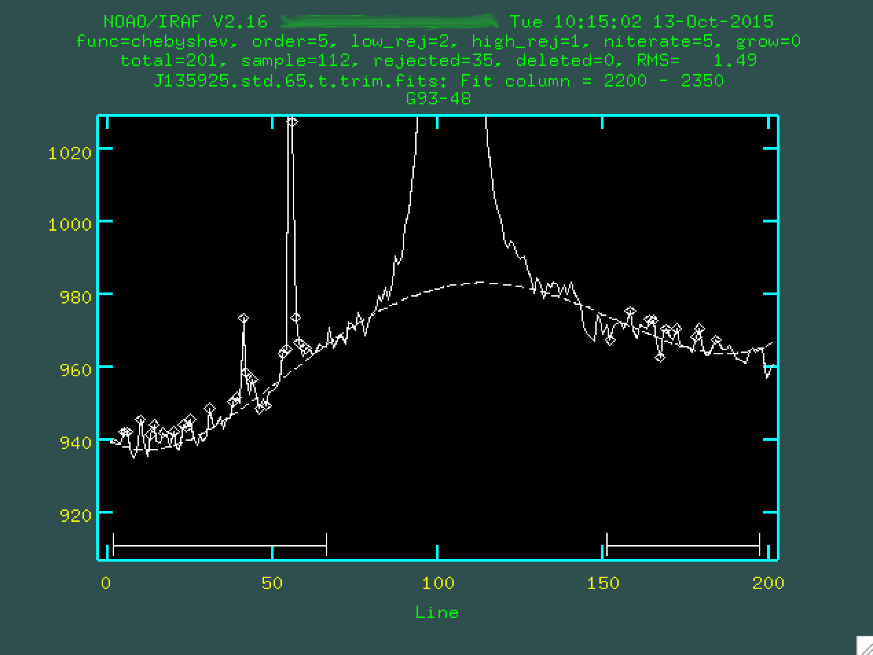
Much better. So, if we're happy with our fit, we can then type q,
and enter, and then background will run, producing our final,
background subtracted image:

This looks good. Next, we have to run the extinction correction. Similar to above, we're going to have to do this by changing the header, first:
> imhead raw_data/mbxgpP201505220065.fits[0] l+
And then find these three keywords:
    EXPTIME =               60.197 / Exposure time
    AIRMASS =     1.21726900642969 / Air mass
    TIME-OBS= '04:33:19.736'       / UTC start of observation
We won't need to update an error spectrum, here, because we don't have one.
The same hedit settings as above will allow
you to update the header, but will ask you before making changes. Run hedit:
     > hedit J135925.std.65.tb.trim.fits EXPTIME 60.197
     > hedit J135925.std.65.tb.trim.fits AIRMASS 1.21726900642969
     > hedit J135925.std.65.tb.trim.fits st "04:33:19.736"
Now, with this done, we'll use the extinction program again:
  > extinction J135925.std.65.tb.trim.fits J135925.std.65.tb.trim.ex.fits
   Extinction correction: J135925.std.65.tb.trim.fits -> J135925.std.65.tb.trim.ex.fits.
Now, it's time to extract the standard star spectrum. You can use the same
parameters as you would when you run the extraction of the actual spectrum.
Just modify the apall.sci.cl script (I rename it
apall.std.cl), and replace the input, output, and final lines of
the script to use the file we just made:
    apall.input="J135925.std.65.tb.trim.ex.fits"
    apall.nfind=1
    apall.output="J135925.std.65.tb.trim.ex.ms.fits"
    apall.apertures=""
    apall.format="multispec"
    apall.references=""
    apall.profiles=""
    ...
    apall J135925.std.65.tb.trim.ex.fits
And then, we run it.
> cl < apall.std.cl
We'll be asked some questions:
  Find apertures for J135925.std.65.tb.trim.ex?  (yes):
  Number of apertures to be found automatically (1):
  Edit apertures for J135925.std.65.tb.trim.ex?  (yes):
As before, we'll be presented with a window showing the central trace, with the standard star aperture selected.
We can go and change the background regions, if we want, byt typing b,
and then deleting the original background regions with z, defining
new regions with s, and refitting with f:
At this point, you want to type q to quit back to the main trace
plot:
And now, if you type q again, the program will ask if you want
to trace the apertures (press enter, as yes should be initially
given as your option), fit the traced positions (again press enter,
as yes should be initially given as your option), and fit a curve to aperture 1
(once more, press enter, as yes should be initially
given as your option).
The first fit to the trace is one dimensional, and so we want to change the
order (I used :or 4) and we may want to delete some of the outlier
points to not influence the fit (with d). Remember to type f
to redo the fit:
And now, armed with this fit, we can extract. Type q, and
apall will ask if you want to write apertures (press enter, again,
if yes is initially given as the option), and extract aperture spectra (press
enter, one last time, if yes is initially given as the option). And now, you
should be able to splot your standard star spectrum:
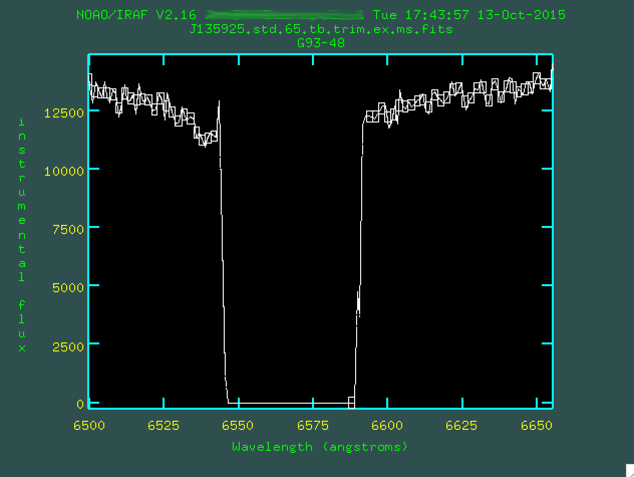
> splot J135925.std.65.tb.trim.ex.ms.fits
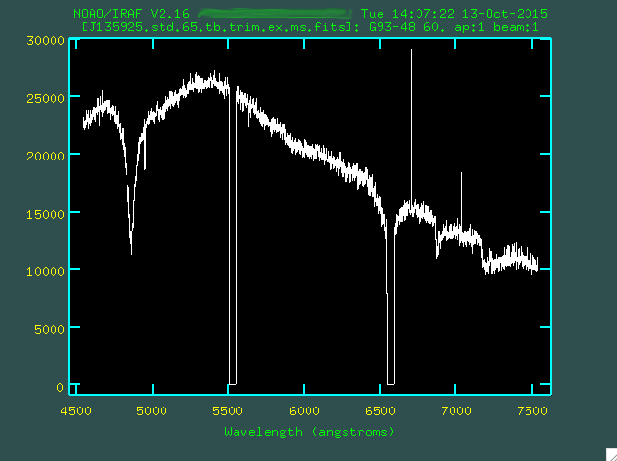
This certainly looks like a chunk of the optical spectrum for this star, from its ESO webpage, doesn't it!
Now, armed with this spectrum, we want to run the flux calibration. Here, I definitely recommend copying over the science spectrum and the standard spectrum to another directory, which you should call "fluxcal," perhaps.
  > mkdir fluxcal
  > cp J135925.std.65.tb.trim.ex.ms.fits fluxcal/
  > cp J135925.med.ex.ms.fits fluxcal/
  > cp J135925.med.sig.ex.ms.fits fluxcal/
  > cd fluxcal/
Now, as discussed on the
OSMOS reduction site I've written, there are standards that are built into
IRAF, which you can find
here (but also you could just type help onedstds and see the
same information in IRAF). Now, the stnadard we're looking at here, G93-48,
is not on this list, so we'll have to go to its
ESO webpage and grab the data files for it there (at the bottom, by clicking
where it says "ftp access to UV+visible
wavelength data files for this standard").
Go ahead and copy the file mg93_48.dat
to your working ("fluxcal") directory. This calibration file should have three
columns: wavelengths (in Angstroms), calibration magnitudes (in AB magnitudes),
and bandpass widths (also in Angstroms).
For the file we download for G93-48, you can see that there are only two columns, however. The third column, with the bandwidth, is not found in the file, so we'll have to kind of fake it. I've written a program, called make_standards_file.pl, which will calculate bandwidths (by just subtracting the wavelengths between individual lines) and produce the new file. You can download this program here, and you can run it in this way (for our standard):
% perl make_standard_file.pl mg93_48.dat > g93_48.dat
Notice that I've named the new file "g93_48.dat," which is the same name
as the star, which is what standard needs, to run the program.
You'll also need to make a file called "standards.men," which says, only:
  Standard stars in this directory

  g93_48
This allows standard to know which standard star you are
referring to. I know that this is all non-ideal, and I welcome any recommendations
on how to do this better.
Now, with everything set up, we can start our flux calibration process,
using the IRAF task standard, which is found in noao.twodspec.longslit.
We should edit one some specific parameters, so let's open up the parameters for
standard, with epar standard:
    PACKAGE = longslit
       TASK = standard

    input   = J135925.std.65.tb.trim.ex.ms.fits  Input image file root name
    output  = J135925.std.65.tb.trim.ex.ms.out  Output flux file (used by SENSFUNC)
    (samesta=                  yes) Same star in all apertures?
    (beam_sw=                   no) Beam switch spectra?
    (apertur=                     ) Aperture selection list
    (bandwid=                INDEF) Bandpass widths
    (bandsep=                INDEF) Bandpass separation
    (fnuzero=  3.6800000000000E-20) Absolute flux zero point
    (extinct= onedstds$ctioextinct.dat) Extinction file
    (caldir =                     ) Directory containing calibration
                                    data
    (observa=       )_.observatory) Observatory for data
    (interac=                  yes) Graphic interaction to define new bandpasses
    (graphic=             stdgraph) Graphics output device
    (cursor =                     ) Graphics cursor input
    star_nam=               g93_48  Star name in calibration list
    airmass =                       Airmass
    exptime =                       Exposure time (seconds)
    mag     =                       Magnitude of star
    magband =                       Magnitude type
    teff    =                       Effective temperature or spectral type
    answer  =                  yes  (no|yes|NO|YES|NO!|YES!)
    (mode   =                   ql)
Notice that I've set the caldir to null:
(caldir = ) Directory containing calibration data
If you type two quotation marks in any parameter line, you'll put in a null value, which indicates that you want to use a file in your current directory. Notice, also, that when you are asked for the star name in the calibration list, give the name of the standard star that corresponds to the file you downloaded.
So, let's run standard:
   Input image file root name (J135925.std.65.tb.trim.ex.ms.fits):
   Output flux file (used by SENSFUNC) (J135925.std.65.tb.trim.ex.ms.out):
   J135925.std.65.tb.trim.ex.ms.fits(1): G93-48
   Star name in calibration list (g93_48):
   J135925.std.65.tb.trim.ex.ms.fits[1]: Edit bandpasses? (no|yes|NO|YES|NO!|YES!) (yes):
This screen will appear:
It's hard to see, but there are actually boxes on this plot, which are
defining the flux for this star as compared to the flux known from the ESO file
for the star. Because of the prominent chip gaps, we want to zoom in on a few
regions and delete outlier boxes. Let's zoom in on the left-most chip gap,
again with w e and e:
There are the boxes. Let's delete the four outlier points using
d.

And we can do this for the second chip gap, as well. Remember, we
zoom out by w n and w m.
Now, after removing the outlier boxes, we can type q and
finish up, creating the file J135925.std.65.tb.trim.ex.ms.out.
Now, we can run the next step, which is sensfunc:
  PACKAGE = longslit
     TASK = sensfunc


  standard= J135925.std.65.tb.trim.ex.ms.out  Input standard star data file (from STANDARD)
  sensitiv=                 sens  Output root sensitivity function imagename
  (apertur=                     ) Aperture selection list
  (ignorea=                  yes) Ignore apertures and make one sensitivity function?
  (logfile=              logfile) Output log for statistics information
  (extinct= onedstds$ctioextinct.dat) Extinction file
  (newexti=          extinct.dat) Output revised extinction file
  (observa=       )_.observatory) Observatory of data
  (functio=              spline3) Fitting function
  (order  =                    5) Order of fit
  (interac=                  yes) Determine sensitivity function interactively?
  (graphs =                   sr) Graphs per frame
  (marks  =       plus cross box) Data mark types (marks deleted added)
  (colors =              2 1 3 4) Colors (lines marks deleted added)
  (cursor =                     ) Graphics cursor input
  (device =             stdgraph) Graphics output device
  answer  =                  yes  (no|yes|NO|YES)
  (mode   =                   ql)
Now, this program is going to take in the out file recently produced, and it will create a sensitivity function (sens.fits). By running the program, you are going to fit a sensitivity function to your out file. It will ask if you want to do this interactively:
  > sensfunc
    Fit aperture 1 interactively? (no|yes|NO|YES) (no|yes|NO|YES) (yes):
Indicate yes. You'll be presented with a window:
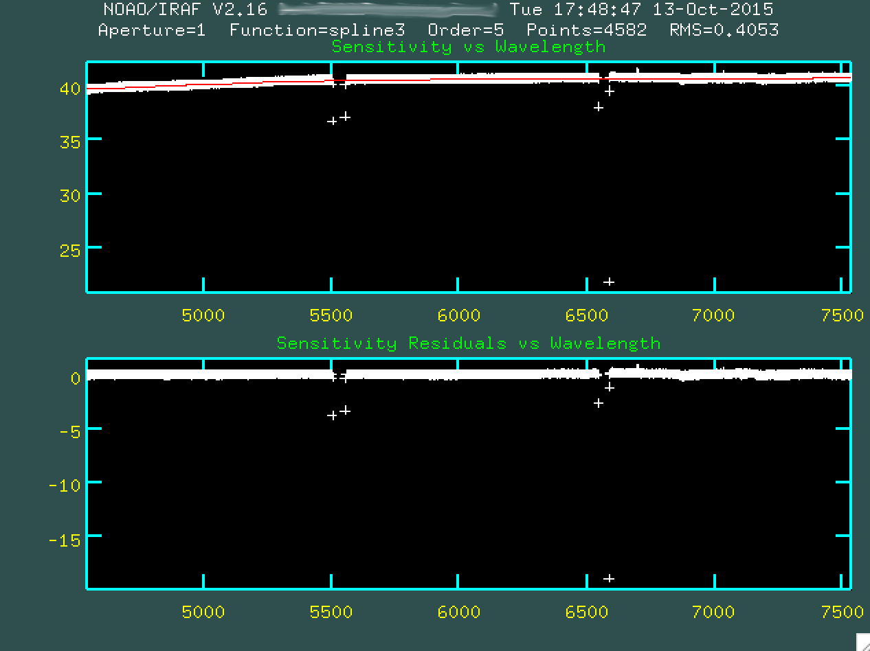
This window shows the sensitivity curve for the instrument based on the
standard star spectrum compared to the internal, correct spectrum for the star.
However, at the moment, due to the chip gaps, it's hard to see the sensitivity
function up close and personal. We can delete the outlier points, right from
the beginning, using d:
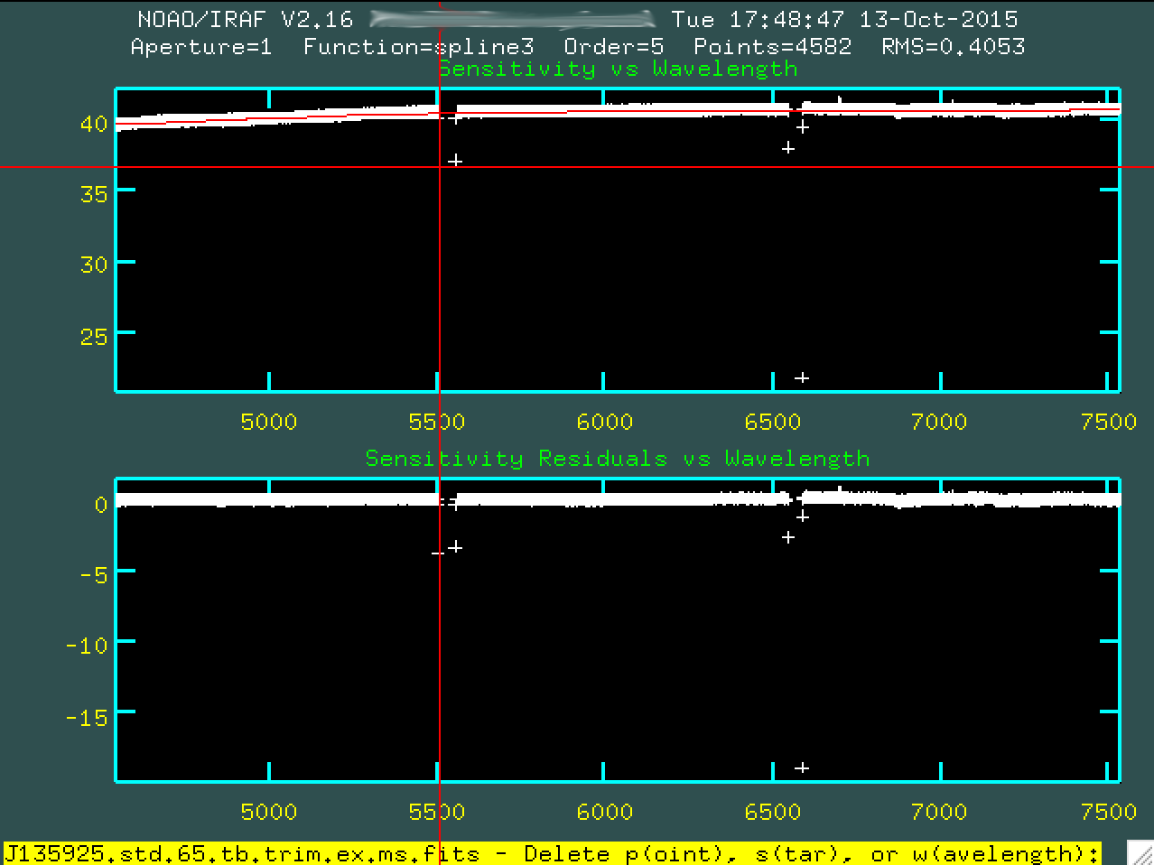
And then pressing p, to indicate we want to delete that point.
Go and do this for all of the outlier points.
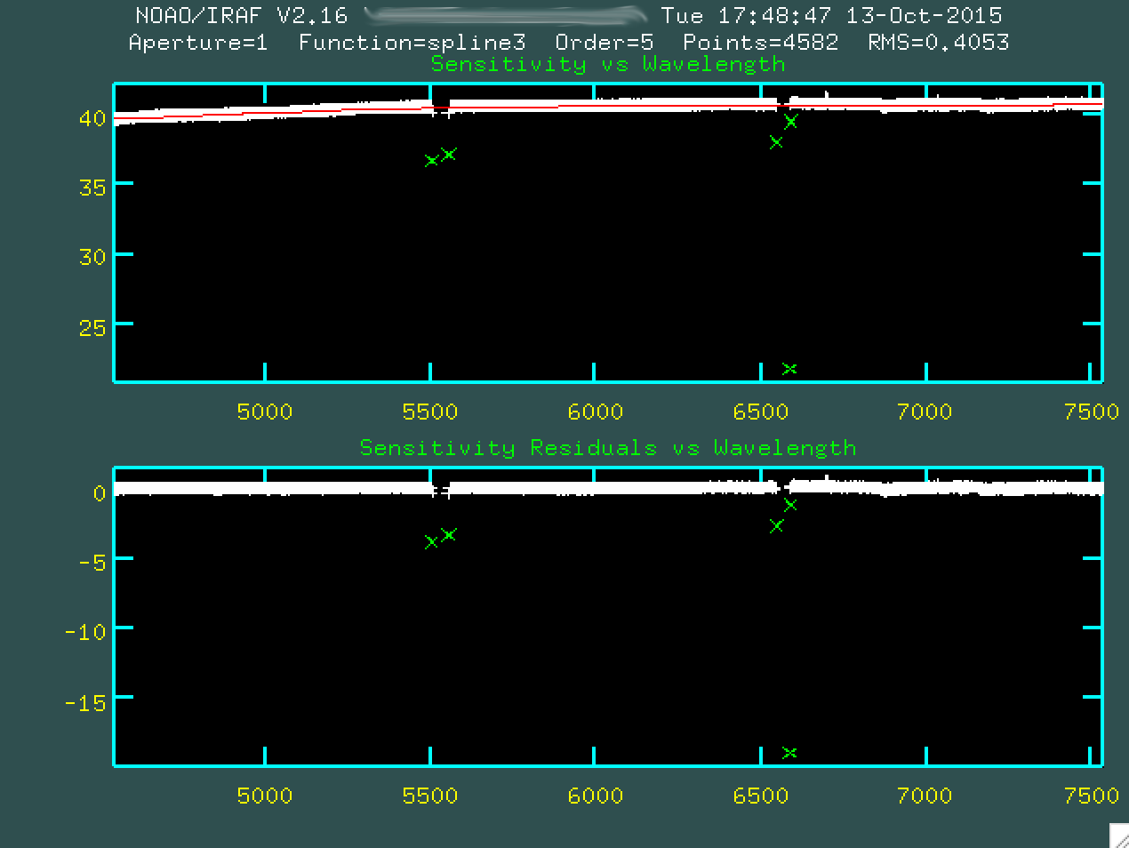
Afterwards, type g to refit and replot the new fit, without
the outlier points. You can't really change the window, since typing w
will change the weights of the nearest point, so you're going to have to stay
zoomed out. As a result, for this, we're going to have to trust that the
sensitivity function is properly fit.
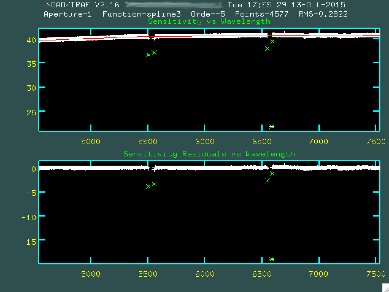
At this point, then, go and type q to quit out, and the
program will produce sens.fits, which is just the fit to that sensitivity
curve you just saw. This will be used to both correct for chip sensitivity
and also to perform a relative flux calibration.
Finally, we can run the flux calibration on our science data. For this,
we'll be running the task calibrate:
  PACKAGE = longslit
     TASK = calibrate

  input   = J135925.med.ex.ms.fits  Input spectra to calibrate
  output  = J135925.med.ex.flam.ms.fits  Output calibrated spectra
  (extinct=                   no) Apply extinction correction?
  (flux   =                  yes) Apply flux calibration?
  (extinct= onedstds$ctioextinct.dat) Extinction file
  (observa=       )_.observatory) Observatory of observation
  (ignorea=                  yes) Ignore aperture numbers in flux calibration?
  (sensiti=                 sens) Image root name for sensitivity spectra
  (fnu    =                   no) Create spectra having units of FNU?
  (mode   =                   ql)
And then we can run things like this:
> calibrate
It's important that you don't apply another extinction correction, but you
do apply a flux calibration, and that you have fnu = no, so the
final flux calibrated spectrum comes out in units of ergs/s/cm^2/Angstrom. You
can convert this to an f_nu (erg/s/cm^2/Hz) by either setting fnu = yes,
or, we could use sarith:
> sarith J135925.med.ex.flam.ms.fits fnu "" J135925.med.ex.fnu.ms.fits
The program sarith requires two inputs and an operator separating
them, but when you're running an operation like fnu, or
sqrt on the spectrum, you just put in "", which
represents "no input", for the second input.
Congrats! Now you have a flux calibrated spectrum! Make sure to run this on the variance spectrum as well!
  PACKAGE = longslit
     TASK = calibrate

  input   = J135925.med.sig.ex.ms.fits  Input spectra to calibrate
  output  = J135925.med.sig.ex.flam.ms.fits  Output calibrated spectra
  (extinct=                   no) Apply extinction correction?
  (flux   =                  yes) Apply flux calibration?
  (extinct= onedstds$ctioextinct.dat) Extinction file
  (observa=       )_.observatory) Observatory of observation
  (ignorea=                  yes) Ignore aperture numbers in flux calibration?
  (sensiti=                 sens) Image root name for sensitivity spectra
  (fnu    =                   no) Create spectra having units of FNU?
  (mode   =                   ql)
And...
> calibrate
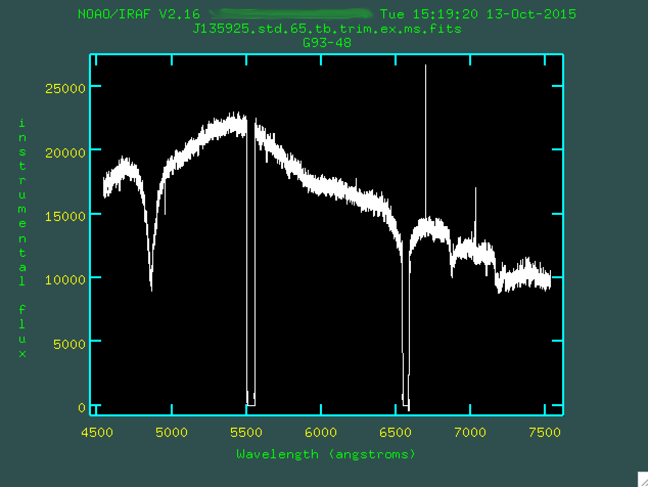
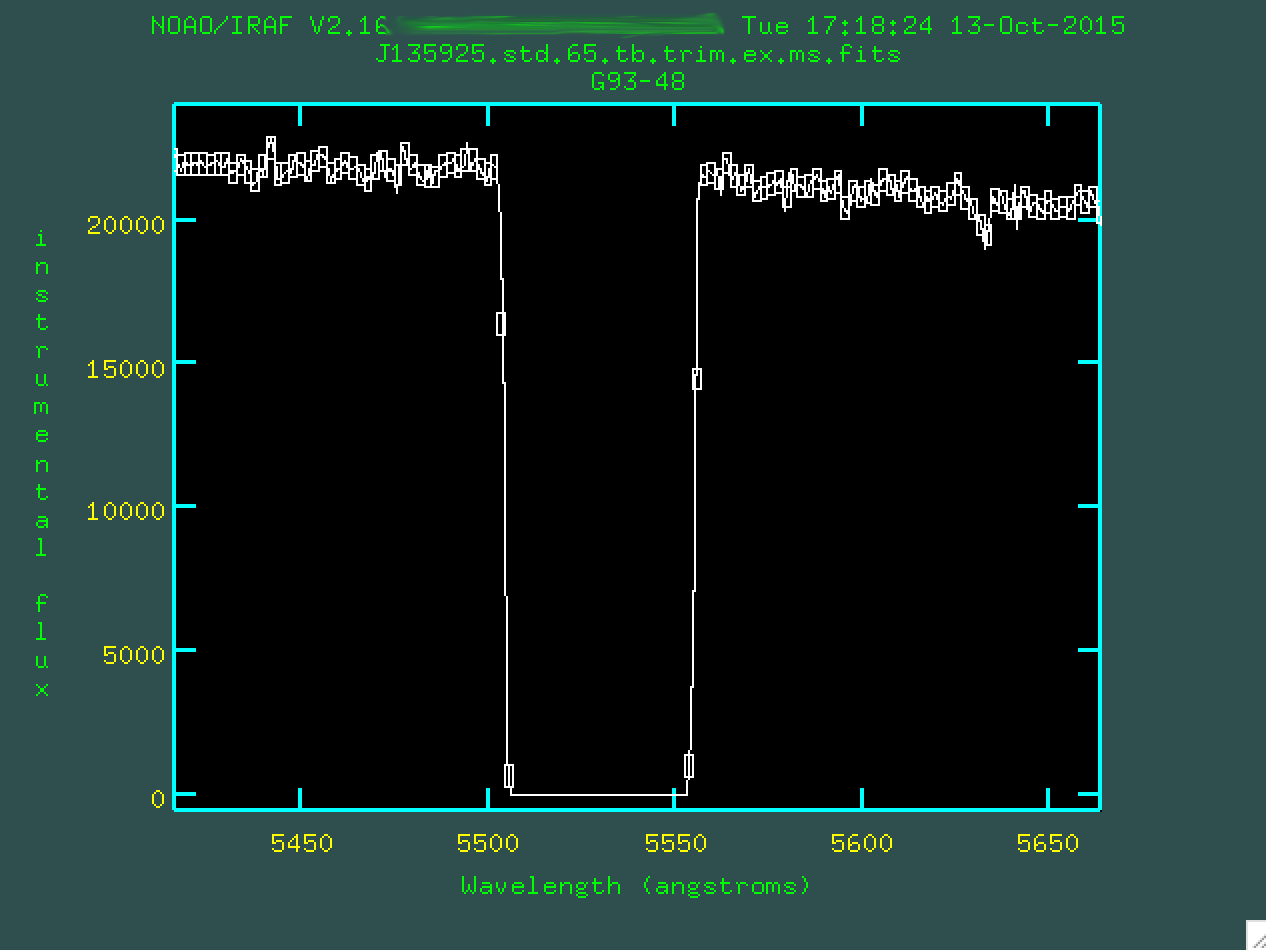
Now, let's take a look at our flux calibrated spectrum:
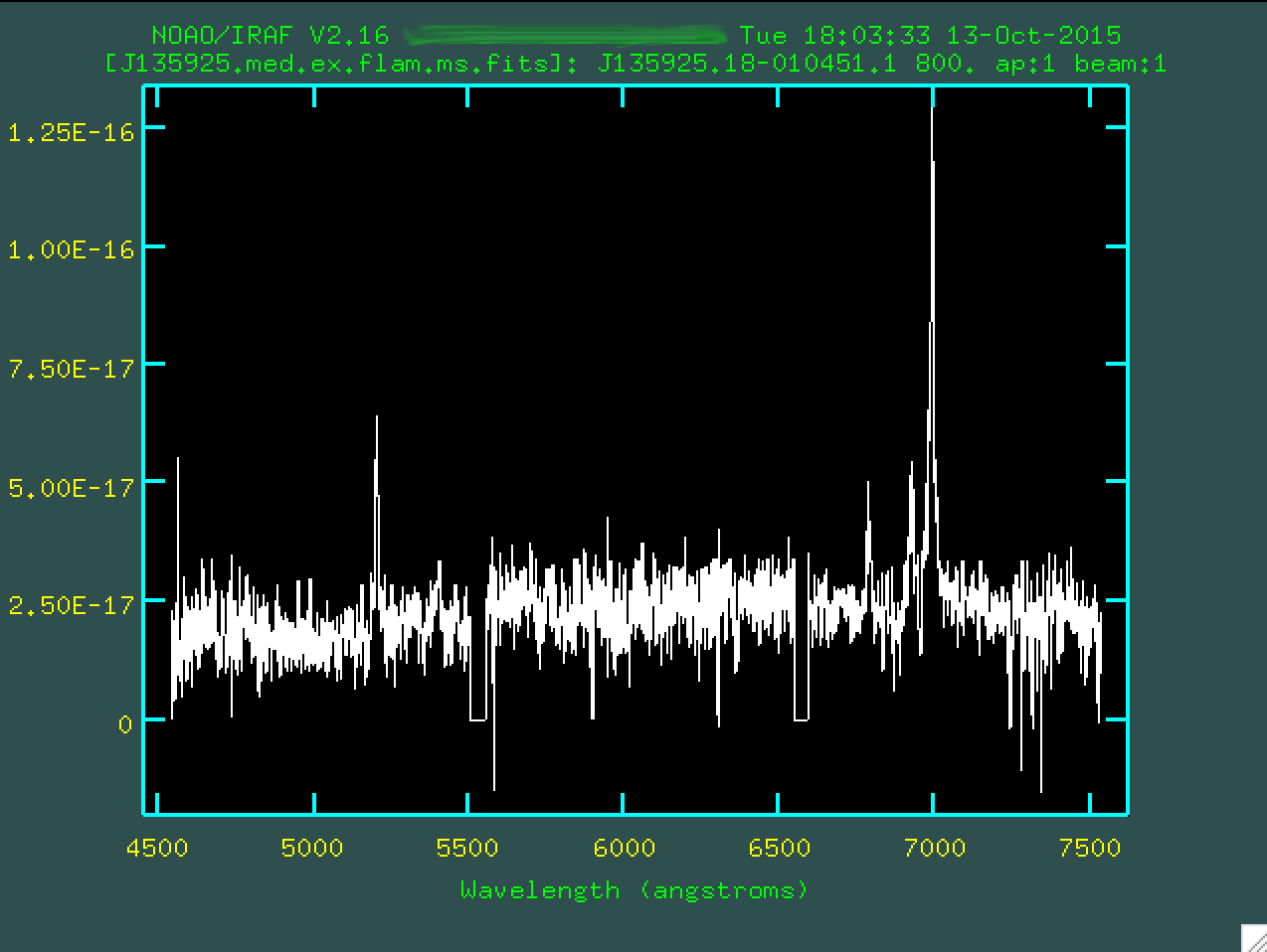
This looks great! We're almost done!
Heliocentric Velocity Correction
Our final step is to correct our spectrum for the motion of the Earth around
the Sun. We are going to use an IRAF program called rvcorrect to
calculate the heliocentric correction, and then we'll use dopcor
to actually shift our spectra. First, rvcorrect requires that you
have two header keywords that are not in our data. First, we need to get the
TIME-OBS from the header, which we did earlier:
> imhead mbxgpP201505180032.fits[0] l+
And it returned:
  RA      = '13:59:25.19       ' / Target RA
  DEC     = '-01:04:51.10      ' / Target declination
  DATE-OBS= '2015-05-18'         / Date of observation
  TIME-OBS= '19:00:37.535'       / UTC start of observation
And now, we should run hedit on the data:
   > hedit J135925.med.ex.flam.ms.fits RA "13:59:25.19"
   > hedit J135925.med.ex.flam.ms.fits DEC "-01:04:51.10"
   > hedit J135925.med.ex.flam.ms.fits UT "19:00:37.535"
   > hedit J135925.med.ex.flam.ms.fits DATE-OBS "2015-05-18"
   > hedit J135925.med.ex.flam.ms.fits EPOCH "2000"
   > hedit J135925.med.ex.flam.ms.fits OBSERVATORY "SAAO"

   > hedit J135925.med.sig.ex.flam.ms.fits RA "13:59:25.19"
   > hedit J135925.med.sig.ex.flam.ms.fits DEC "-01:04:51.10"
   > hedit J135925.med.sig.ex.flam.ms.fits UT "19:00:37.535"
   > hedit J135925.med.sig.ex.flam.ms.fits DATE-OBS "2015-05-18"
   > hedit J135925.med.sig.ex.flam.ms.fits EPOCH "2000"
   > hedit J135925.med.sig.ex.flam.ms.fits OBSERVATORY "SAAO"
So, we had to add RA, DEC, DATE-OBS, UT, EPOCH, and OBSERVATORY to the
header. Once we've done that, we can run rvcorrect:
> rvcorrect images=J135925.med.ex.flam.ms.fits
And we are presented with:
  # RVCORRECT: Observatory parameters for South African Astronomical Observatory
  #       latitude = -32:22:46
  #       longitude = 339:11:21.5
  #       altitude = 1798
  ##   HJD          VOBS   VHELIO     VLSR   VDIURNAL   VLUNAR  VANNUAL   VSOLAR
  2457161.29711     0.00   -13.63    -5.45      0.184   -0.008  -13.802    8.179
The most important number is VHELIO, which gives the heliocentric
velocity that we have to correct for, using dopcor, found in
noao.twodspec.longslit:
   > dopcor J135925.med.ex.flam.ms.fits J135925.med.exhel.flam.ms.fits 13.63 isvel+
   > dopcor J135925.med.sig.ex.flam.ms.fits J135925.med.sig.exhel.flam.ms.fits 13.63 isvel+
We'll use the the negative of the VHELIO value in order to correct for the heliocentric motion. We've also applied the same correction to the extinction corrected, flux calibrated sigma spectrum as well.
And so that's it! We now have reduced, flux calibrated, extinction and heliocentric velocity spectra, with units of F_lambda vs. Angstrom. Perfect for measuring emission line fluxes! Good luck!